广义加性模型Generalized additive models-pyGAM的使用

目录1 安装pyGAM2 分类案例2.1 基本使用2.2 部分依赖图（Partial dependency plots）2.3 调整光滑度和惩罚2.4 自动调参3 完整的pyGAM模型4 测试参数4.1 测试惩罚项4.2 测试样条函数的数量4.3 测试不同的约束5 小问题1 安装pyGAMpip install pygam在statsmodels.api中，也有GAM相关包。比如from.....

Alex Tech Bolg

13016人浏览 · 2020-03-06 01:14:38

Alex Tech Bolg · 2020-03-06 01:14:38 发布

0 代码示例

全部代码示例请参考：

https://github.com/Alex2Yang97/Learning_tutorials/tree/main/gam_model

1 安装pyGAM

pip install pygam

在statsmodels.api中，也有GAM相关包。比如

from statsmodels.gam.api import GLMGam, BSplines

2 分类案例

2.1 基本使用

我们使用LogisticGAM来进行分类处理，通过load_breast_cancer来导入数据。

import pandas as pd        
from pygam import LogisticGAM
from sklearn.datasets import load_breast_cancer

#load the breast cancer data set
data = load_breast_cancer()

#keep first 6 features only
df = pd.DataFrame(data.data, columns=data.feature_names)[['mean radius', 'mean texture', 'mean perimeter', 'mean area','mean smoothness', 'mean compactness']]
target_df = pd.Series(data.target)
df.describe()

建立模型。

X = df[['mean radius', 'mean texture', 'mean perimeter', 'mean area','mean smoothness', 'mean compactness']]
y = target_df
#Fit a model with the default parameters
gam = LogisticGAM().fit(X, y)

查看结果。summary()提供了很多统计量，比如AIC，UBRE，修正R^2。

gam.summary()

查看拟合准确率。

gam.accuracy(X, y)

2.2 部分依赖图（Partial dependency plots）

gam的优势之一是，gam的可加性让我们能够控制其他变量，来探究和解释某一个变量。通过generate_X_grid来帮助我们产生合适的画图数据。

lt.rcParams['figure.figsize'] = (28, 8)
fig, axs = plt.subplots(1, len(data.feature_names[0:6]))
titles = data.feature_names

for i, ax in enumerate(axs):
    XX = gam.generate_X_grid(term=i)
    ax.plot(XX[:, i], gam.partial_dependence(term=i, X=XX))
    ax.plot(XX[:, i], gam.partial_dependence(term=i, X=XX,   width=.95)[1], c='r', ls='--')
    ax.set_title(titles[i])
plt.show()

部分依赖图
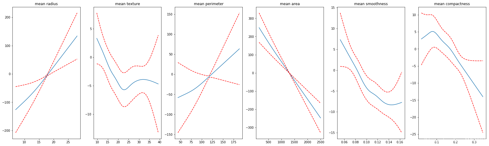
我们能够看到一些有趣的结果，有一些变量和目标值之间有非常明显简单的线性关系；但是有一些变量和目标值之间有着很强的非线性关系。我们非常想要结合这些图像的可解释性，并且防止GAM过拟合，从而提出一个能够推广到持久数据集的模型。

部分依赖图（Partial dependency plots）非常有用，因为他们具有高度的可解释性，并且易于理解。比如，在第一个测试结果中，我们可以说the mean radius of the tumor 和the response variable具有很强的关系；the mean radius of the tumor越大，是malignant（恶性）的可能性越大。

对于其他的特征，比如the mean texture很难解释，并且我们已经推断我们希望有一条更平滑的曲线。（我的理解是，有先验知识的情况下，我们通过设置约束，强制让某一个特征对目标值有着单调递增或递减的特性，或者调整样条函数的数量。）

2.3 调整光滑度和惩罚

主要调整的参数有三个，n_splines，lam，和constraints。

n_splines：用来拟合的spline函数（样条函数）的数量
lam：惩罚项（在整个目标函数中乘以二阶导数）
constraints：允许用户指定函数是否应具有单调约束的约束列表。包括[‘convex’, ‘concave’, ‘monotonic_inc’, ‘monotonic_dec’,’circular’, ‘none’]

默认情况下：

n_splines = 25
lam = 0.6
constraints = None

更改n_splines让曲线变得更光滑。（值得注意的是，如果惩罚项，如果对于每一个特征都是一样的值，则不需要写成list形式；如果不一样的值，那么可以写成列表）

lambda_ = 0.6
n_splines = [25, 6, 25, 25, 6, 4] 
constraints = None
gam = LogisticGAM(constraints=constraints, 
          lam=lambda_,
         n_splines=n_splines).fit(X, y)

画出图像后，可以看到，之前不平滑的特征部分依赖图（partial dependency plots）变得平滑了。
部分依赖图2
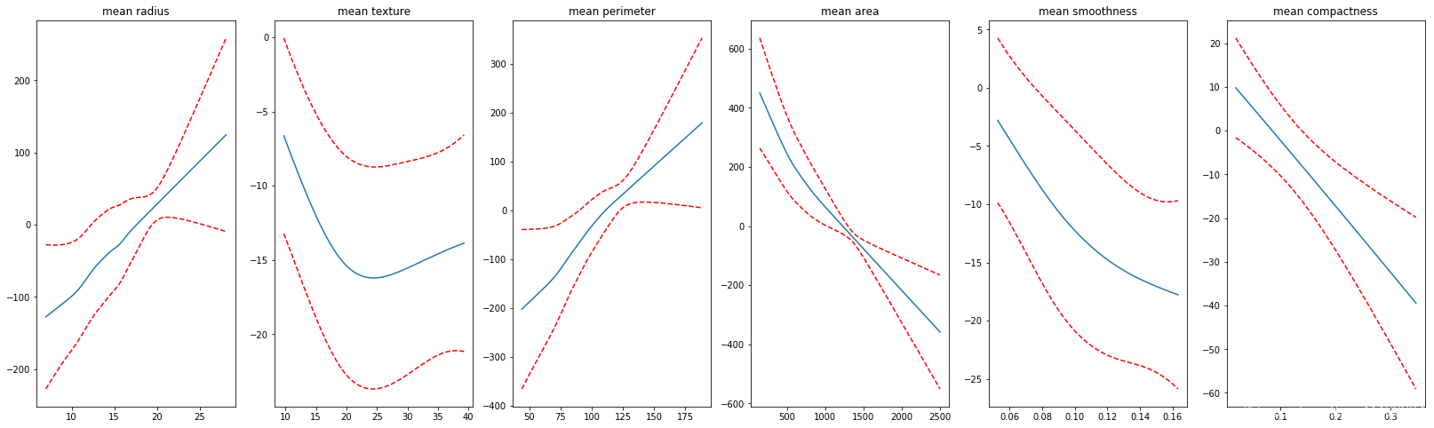
如果我们强制平滑后，准确度下降了，说明我们损失了一部分信息（没有捕捉到部分信息），不过同样，准确度的下降也表明我们可以将多少我们的直觉加入到模型中。

参数lam控制着惩罚程度，就算我们将n_splines设置的很大，但是惩罚很大的话，函数图像可能仍然会出现直线。

2.4 自动调参

通过gridsearch来自动选择参数。默认参数是一个字典类型的lam，{‘lam’:np.logspace(-3,3,11)}

gam = LogisticGAM().gridsearch(X, y)

有三种方式：

1、通过网格，将grid变成list，搜寻的数量一共有2**6个。（6个特征）

>>> lam = np.logspace(-3, 3, 2)
>>> lams = [lam] * 6
>>> gam.gridsearch(X, y, lam=lams)

2、直接将网格变成np.ndarray，当搜索的空间非常大的时候，我们会随机进行搜索。

>>> lams = np.exp(np.random.random(50, 4) * 6 - 3)
>>> gam.gridsearch(X, y, lam=lams)

3、copying grids for parameters with multiple dimensions. if we specify a 1D np.ndarray for lam, we are implicitly testing the space where all points have the same value

>>> gam.gridsearch(lam=np.logspace(-3, 3, 11))

或者

>>> lam = np.logspace(-3, 3, 11)
>>> lams = np.array([lam] * 4)
>>> gam.gridsearch(X, y, lam=lams)

3 完整的pyGAM模型

使用留出数据集是最好的权衡模型的偏差-方差的方法。pyGAM很好地适应sklearn的工作流程，因此这一步骤很像拟合sklearn模型。

首先是分离训练集和测试机。

import numpy as np
from sklearn.model_selection import train_test_split
X_train, X_test, y_train, y_test = train_test_split(X, y, test_size=0.33, random_state=42)
gam = LogisticGAM().gridsearch(X_train, y_train)

预测。

from sklearn.metrics import accuracy_score
from sklearn.metrics import log_loss
predictions = gam.predict(X_test)
print("Accuracy: {} ".format(accuracy_score(y_test, predictions)))
probas = gam.predict_proba(X_test)      
print("Log Loss: {} ".format(log_loss(y_test, probas))

下面，减小样条函数（spline）的数量，来看一下准确率。

lambda_ = [0.6, 0.6, 0.6, 0.6, 0.6, 0.6]
n_splines = [4, 14, 4, 6, 12, 12] 
constraints = [None, None, None, None, None, None]
X_train, X_test, y_train, y_test = train_test_split(X, y, test_size=0.33, random_state=42)
gam = LogisticGAM(constraints=constraints, 
                  lam=lambda_,
                 n_splines=n_splines).train(X_train, y_train)
predictions = gam.predict(X_test)
print("Accuracy: {} ".format(accuracy_score(y_test, predictions)))
probas = gam.predict_proba(X_test)      
print("Log Loss: {} ".format(log_loss(y_test, probas)))

4 测试参数

使用LinearGAM，进行测试。

from sklearn.datasets import load_boston
from pygam import LinearGAM

boston = load_boston()
df = pd.DataFrame(boston.data, columns=boston.feature_names)
target_df = pd.Series(boston.target)
df.head()

4.1 测试惩罚项

lambda_list = [0.01, 0.1, 1, 10, 100]
for lambda_ in lambda_list:
    constraints = None
    gam = LinearGAM(constraints=constraints, 
                    lam=lambda_).fit(X.values, y)
    print(f'\nlambda_: {lambda_}')
    plot_feature_plot(gam)

测试1
测试2

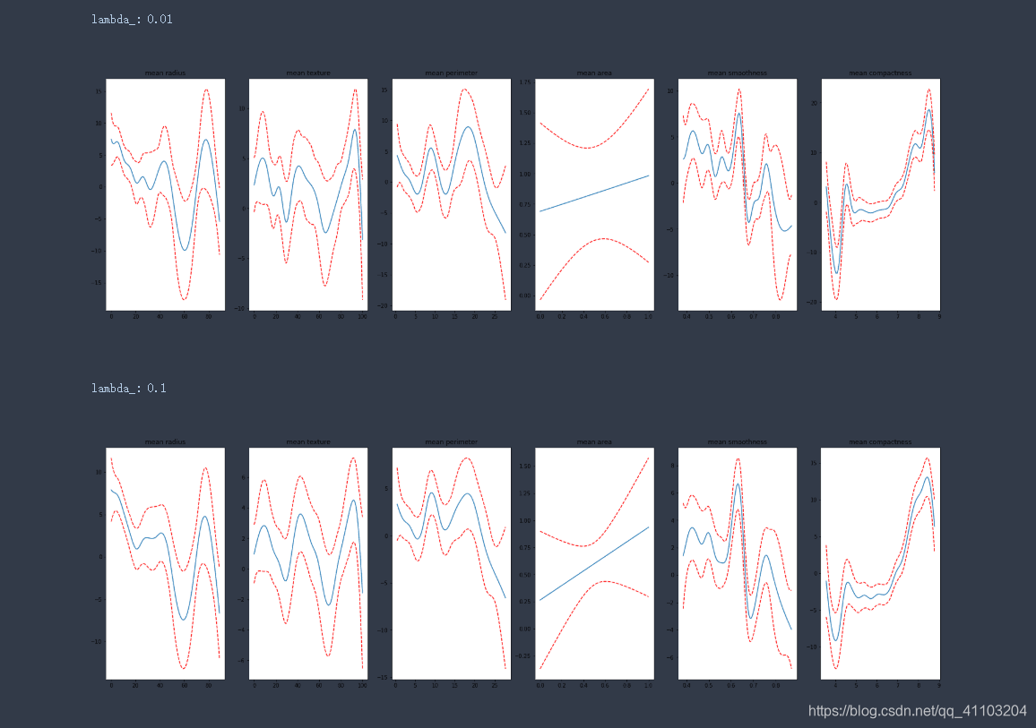
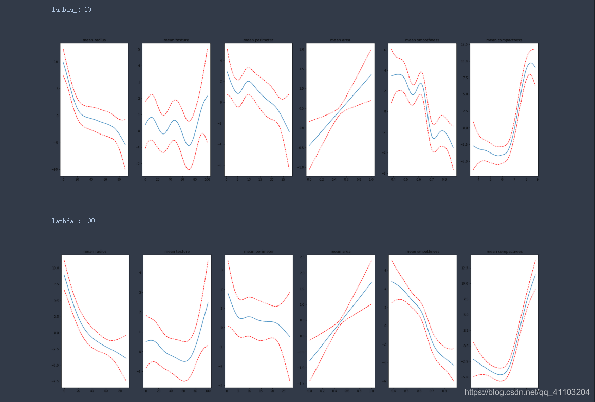
根据图像可以看出，惩罚越大，拟合的曲线越平滑。

4.2 测试样条函数的数量

n_splines_list = [[4]*13, [10]*13, [100]*13, [1000]*13]
for n_splines in n_splines_list:
    constraints = None
    gam = LinearGAM(constraints = constraints, 
                    n_splines = n_splines).fit(X.values, y)
    print(f'\nlambda_: {n_splines}')
    plot_feature_plot(gam)

4,10
2-2
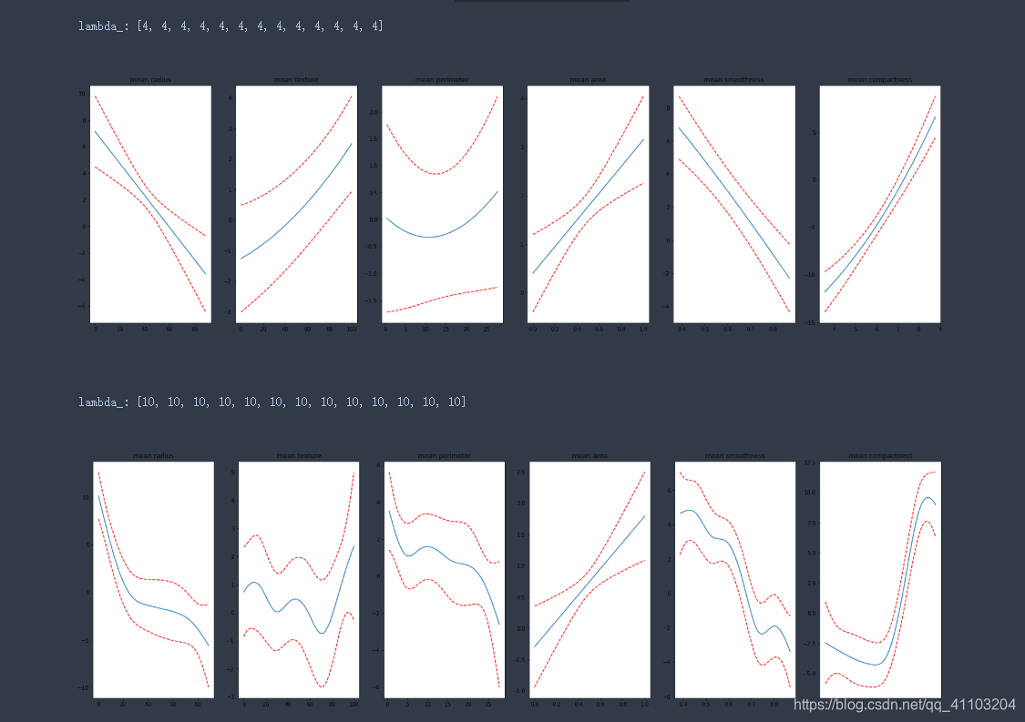
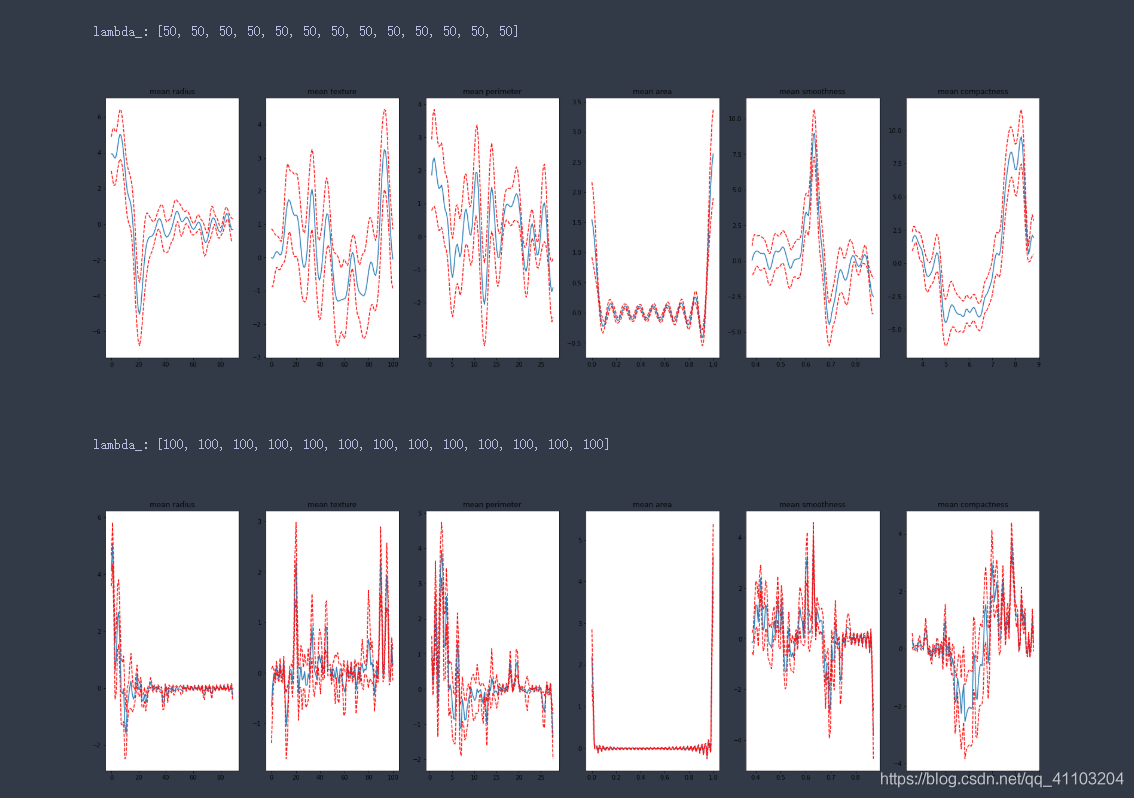
样条函数越多，拟合越好，但是过多之后，会出现过拟合。

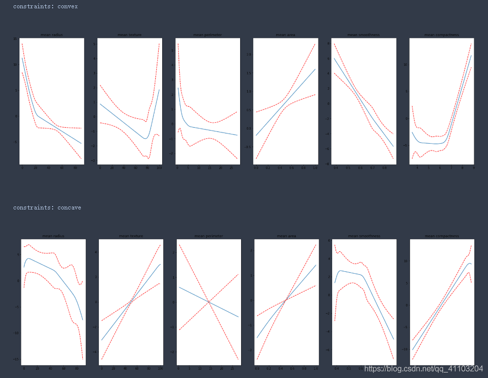
4.3 测试不同的约束

constraints_list = ['convex', 'concave', 'monotonic_inc', 'monotonic_dec', 'none']# circular这里无法使用
for constraints in constraints_list:
    gam = LinearGAM(constraints = constraints).fit(X.values, y)
    print(f'\nconstraints: {constraints}')
    plot_feature_plot(gam)