Glcm 灰度共生矩阵,保姆级别教程,获取图片的Glcm和基于Glcm的纹理特征,附讲解思路,python代码的实现
保姆级别教程,获取图片的Glcm和基于Glcm的纹理特征,附讲解思路,python代码的实现网络上Glcm的原理很多,但是实现的python代码我确实没找到,讲的也不是很清楚此文介绍了如何在一张图片中得到Glcm灰度共生矩阵,并基于Glcm的特征提取.带每一步的讲解Glcm(Gray-level co-occurrence matrix) 灰度共生矩阵原理:就是通过计算灰度图像得到它的共生矩阵,然
保姆级别教程,获取图片的Glcm和基于Glcm的纹理特征,附讲解思路,python代码的实现
网络上Glcm的原理很多,但是实现的python代码我确实没找到,讲的也不是很清楚
此文介绍了如何在一张图片中得到Glcm灰度共生矩阵,并基于Glcm的特征提取.带每一步的讲解
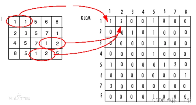
Glcm(Gray-level co-occurrence matrix) 灰度共生矩阵
原理:就是通过计算灰度图像得到它的共生矩阵,然后透过计算这个共生矩阵得到矩阵的部分特征值,来分别代表图像的某些纹理特征(纹理的定义仍是难点)。
灰度共生矩阵能反映图像灰度关于方向、相邻间隔、变化幅度的综合信息,它是分析图像的局部模式和它们排列规则的基础.
明确几个概念:方向,偏移量和灰度共生矩阵的阶数.
定义:灰度共生矩阵是图像中相距为D的两个灰度像素同时出现的联合概率分布.
意义:共生矩阵方法用条件概率来反映纹理,是相邻像素的灰度相关性的表现.

步骤:
1.opencv 读取图片 调用库cv2
2.调用skimage 的feature文件中的greycomatrix, greycoprops函数
3.将图片划分为 8个等级的灰度共生矩阵
4.依据灰度共生矩阵获得图片的特征量
import numpy as np
from skimage.feature import greycomatrix, greycoprops
import cv2
import os
import matplotlib.pyplot as plt
from matplotlib.font_manager import FontProperties
font = FontProperties(fname=r"c:\windows\fonts\simsun.ttc", size=16) #导入本地汉字字库,pyplot显示中文
1.测试greycomatrix函数 256阶 化为 8个等级
gray = np.random.randint(0,255,(10,10))
gray,gray.shape
'''将图片的256阶化为 8个等级'''
gray_8 = (gray/32).astype(np.int32)
gray,gray_8
(array([[ 46, 221, 101, 155, 36, 46, 192, 102, 140, 197],
[213, 47, 202, 246, 120, 204, 201, 131, 202, 1],
[117, 52, 230, 225, 23, 249, 215, 154, 216, 225],
[ 19, 218, 26, 92, 77, 209, 165, 206, 195, 17],
[ 93, 116, 12, 82, 130, 225, 195, 172, 249, 39],
[ 20, 41, 204, 144, 37, 186, 25, 47, 54, 100],
[245, 238, 100, 91, 143, 243, 229, 180, 71, 190],
[175, 0, 62, 218, 173, 154, 80, 51, 233, 28],
[ 98, 115, 254, 52, 165, 250, 147, 237, 47, 246],
[126, 156, 246, 39, 140, 119, 25, 242, 1, 198]]),
array([[1, 6, 3, 4, 1, 1, 6, 3, 4, 6],
[6, 1, 6, 7, 3, 6, 6, 4, 6, 0],
[3, 1, 7, 7, 0, 7, 6, 4, 6, 7],
[0, 6, 0, 2, 2, 6, 5, 6, 6, 0],
[2, 3, 0, 2, 4, 7, 6, 5, 7, 1],
[0, 1, 6, 4, 1, 5, 0, 1, 1, 3],
[7, 7, 3, 2, 4, 7, 7, 5, 2, 5],
[5, 0, 1, 6, 5, 4, 2, 1, 7, 0],
[3, 3, 7, 1, 5, 7, 4, 7, 1, 7],
[3, 4, 7, 1, 4, 3, 0, 7, 0, 6]]))
函数详解:包含主要4个参数 图片,距离(需要为列表),角度(列表),灰度等级
greycomatrix(image, distances, angles, levels=None, symmetric=False,
normed=False)
symmetric :
如果为真,则输出矩阵P[:, :, d, theta]是对称的。这一点是通过忽略数值对的顺序来实现的.
normed:
如果是 “真”,则对每个矩阵P[:, :, d, theta]进行规范化处理,方法是将其除以
除以给定偏移量的累计共现总数。
偏移量。所得矩阵的元素之和为1。
默认为假.
传参要求
:greycomatrix(image, [1], [0, np.pi/4, np.pi/2, 3*np.pi/4],
… levels=4
levels:级别数应该大于图像中的最大灰度值.
返回值:
P : 4-D ndarray
The grey-level co-occurrence histogram. The value
P[i,j,d,theta] is the number of times that grey-level j
occurs at a distance d and at an angle theta from
grey-level i. If normed is False, the output is of
type uint32, otherwise it is float64. The dimensions are:
levels x levels x number of distances x number of angles.
如下,调用灰度共生矩阵,传入参数,获得一个8灰阶的 8x8灰度共生矩阵
距离[1] 角度[0]
Glcm = greycomatrix(gray_8,[1],[0],levels=8)
Glcm_1 = Glcm.squeeze()
Glcm_1.shape,Glcm_1
((8, 8),
array([[0, 3, 2, 0, 0, 0, 2, 2],
[0, 2, 0, 1, 1, 2, 5, 3],
[0, 1, 1, 1, 2, 1, 1, 0],
[2, 1, 1, 1, 3, 0, 1, 1],
[0, 2, 1, 1, 0, 0, 3, 4],
[2, 0, 1, 0, 1, 0, 1, 2],
[3, 1, 0, 2, 3, 3, 2, 2],
[3, 4, 0, 2, 1, 1, 2, 3]], dtype=uint32))
{‘contrast’, ‘dissimilarity’,
‘homogeneity’, ‘energy’, ‘correlation’, ‘ASM’}
也就是一个Glcm 矩阵会 得到一个值
temp = greycoprops(Glcm,'ASM')
temp.shape,temp
((1, 1), array([[0.02691358]]))
def cut_img_step(img,step): # 每个块大小为20x20
'''传入Gray 图片与 step'''
new_img = [] #240x240
for i in np.arange(0, img.shape[0] + 1, step):
for j in np.arange(0, img.shape[1] + 1, step):
if i + step <= img.shape[0] and j + step <= img.shape[1]:
new_img.append(img[i:i + step, j:j + step])
new_img = np.array(new_img, dtype=np.int32)
return new_img
好了,正式开始获取一张图片的Glcm 纹理
pwd = os.getcwd()
pwd
'D:\\_py项目文件夹\\ML-opencv-sklearn\\machine-book\\特征算子学习'
img = cv2.imread(r"../figures/guangzhou tower.jpg",cv2.IMREAD_GRAYSCALE)
'''将原图片的256阶化为 64个等级'''
level = 64
scale_data = 256/level
img_64= (img / scale_data).astype(np.int32)
plt.subplot(211)
plt.imshow(img,cmap='gray')
plt.title("256阶 675x1200",fontproperties=font)
plt.axis("off")
plt.subplot(212)
plt.imshow(img_64,cmap='gray')
plt.title("64阶 675x1200",fontproperties = font)
plt.axis("off")
plt.show()

如上图所示,我们使用了一张广州塔的图片,图片
Height, width
(675,1200)
这里要注意:
Float images are not supported by greycomatrix. Convert the image to an unsigned integer type.
opencv 读取图片会是float32这里需要将img_64 转为uint8类型
'''获取整张图片的Glcm纹理 4个方向 0-》3/4 pi,64阶'''
img_glcm64 = greycomatrix(img_64, [1], [0, np.pi / 4, np.pi / 2, 3 * np.pi / 4], levels=level)
'''将四个灰度共生矩阵对应相加后取
平均数得到影像的综合灰度共生矩阵'''
mean = []
for g_level1 in img_glcm64:
for g_level2 in g_level1:
for i in g_level2:
mean.append(np.mean(i))
mean = np.array(mean)
'''Glcm_new 中保存了原图的Glcm4个方向的平均值'''
Glcm_new = mean.reshape(( level, level,1,1))# 后两个参数为步长数,方向数,计算特征需要
plt.subplot(211)
plt.imshow(img_64,cmap='gray')
plt.title("64阶 675x1200",fontproperties=font)
plt.axis("off")
plt.subplot(212)
plt.imshow(Glcm_new.reshape(level,level),cmap='gray')
plt.title("64阶Glcm 64x64",fontproperties = font)
plt.axis("off")
plt.show()

对角附近的元素有较大的值,说明图像的像素具有相似的像素值,
如果偏离对角线的元素会有比较大的值,说明像素灰度在局部有较大变化.
如上图,由于glcm 是一个统计量,如果我们使用pyplot 来显示图片,那么这个图片的信息实际是蕴含了一个三维的信息
[x轴,y轴,z轴],z轴是一个亮度值,x,y告诉我们位置信息
故而我们可以由这个统计的glcm分析得知,数据主要在主对角线上,也就说明
距离为1,原图4个方向上 有灰度对(x,x)的像素占绝大多少
依据Glcm提取这张图片的特征信息:
{‘contrast’, ‘dissimilarity’, ‘homogeneity’, ‘energy’, ‘correlation’, ‘ASM’}
'''注意greycoprops的传参要求 glcm 需要为[i,j,d,theta] '''
features = []
for prop in {'contrast', 'dissimilarity', 'homogeneity', 'energy', 'correlation', 'ASM'}:
features.append(greycoprops(Glcm_new, prop))#
features
[array([[0.0107847]]),
array([[1.20763164]]),
array([[0.10384942]]),
array([[11.31592761]]),
array([[0.7139315]]),
array([[0.96871746]])]
此时我们提取了这张图片,基于glcm 的特征
提取特征后,可以使用svm支持向量机来进行分类或者其他工作
如果说觉得一张图片只是取6个特征值有点少,那咱们也可以通过其他操作来增加特征的维度
1.通过分割图片.获取特征
2.通过特征融合增加其他特征,例如灰度值
以下分享一些自己造的一些轮子
def get_glcm_sixFeature(IMG_gray): # 传入灰度图像
input = IMG_gray # 读取图像,灰度模式
# 得到共生矩阵,参数:图像矩阵,距离,方向,灰度级别,是否对称,是否标准化
glcm = greycomatrix(input,
[1,2],
[0, np.pi / 4, np.pi / 2, np.pi * 3 / 4],
levels=256, symmetric=True,
normed=True) # 100x100 -> 3x4
# 得到共生矩阵统计值,官方文档
# http://tonysyu.github.io/scikit-image/api/skimage.feature.html#skimage.feature.greycoprops
feature = []
feature_descrip = {'contrast', 'dissimilarity',
'homogeneity', 'energy', 'correlation', 'ASM'}
for prop in {'contrast', 'correlation',
'ASM','homogeneity' }:
temp = greycoprops(glcm, prop)
feature.append(temp)
return np.array(feature), glcm
def get_gray_feature(Imgs,step= 25):
'''格式要求 (x灰度图像二维,100,100)'''
print(f"Imgs shape is {Imgs.shape}") #
Imgs_number = Imgs.shape[0]
Gray_feature_num = int((Imgs.shape[1] /step)**2)
Avg_gray = []
for img in Imgs:
cut = cut_img_step(img,step)
for patch in cut: # 每张图4个patch
Avg_gray.append(np.mean(patch))
Avg_gray = np.array(Avg_gray)
Avg_gray = Avg_gray.reshape(Imgs_number, Gray_feature_num)
print(f'Avg_gray shape :{Avg_gray.shape}')
return Avg_gray
其他文章
Sober算子边缘检测与Harris角点检测1
HOG特征+SVM 进行行人检测,带源码,异常处理
线性回归预测波士顿房价

华为开发者空间,是为全球开发者打造的专属开发空间,汇聚了华为优质开发资源及工具,致力于让每一位开发者拥有一台云主机,基于华为根生态开发、创新。
更多推荐


 15
15 1
1- 0


 已为社区贡献2条内容
 免费领云主机


 华为云 x DeepSeek:AI驱动云上应用创新

 DTT年度收官盛典:华为开发者空间大咖汇,共探云端开发创新
 华为云数字人,助力行业数字化业务创新
 企业数据治理一站式解决方案及应用实践
 轻松构建AIoT智能场景应用


所有评论(0)