Python业务分析实战|共享单车数据挖掘
本文详细介绍了共享单车数据挖掘,包括数据分析和模型开发。它包含以下步骤:共享单车数据挖掘数据集简介关于共享单车数据集自行车共享系统是传统自行车租赁的新一代,从注册会员、租赁到归还的整个过程...
本文详细介绍了共享单车数据挖掘,包括数据分析和模型开发。它包含以下步骤:

数据集简介
关于共享单车数据集
自行车共享系统是传统自行车租赁的新一代,从注册会员、租赁到归还的整个过程都是自动化的。通过这些系统,用户可以很容易地从一个特定的位置租用自行车,并在另一个位置归还。目前,全球大约有500多个共享单车项目,这些项目由50多万辆自行车组成。今天,由于它们在交通、环境和健康问题上的重要作用,人们对这些系统产生了极大的兴趣。
除了自行车共享系统在现实世界的有趣应用之外,众多研究者们对这些系统所产生的数据产生浓厚的兴趣。与其他运输服务(如公共汽车或地铁)不同,共享自行车使用的持续时间、出发时间和到达位置都明确地记录在系统中。这一功能将自行车共享系统变成了一个虚拟传感器网络,可用于感知城市中的流动性。因此,通过监测这些数据,预计可以检测到城市中的大多数重要事件。
今天我们就运用这些数据集,挖掘出蕴含在其中的有效的信息。接下来从探索数据属性,清洗数据,到模型开发,一起来学习,共同进步。
注意,该数据集是国外共享单车数据集,并非国内的共享单车数据集。但不影响我们学习数据挖掘相关知识和技术。数据集获取可以联系原文作者云朵君(Mr_cloud_data)获取。
属性信息
hour.csv和 day.csv都有以下字段,day.csv中没有 hr 字段
instant:记录索引dteday:日期season:季节 (1:春天, 2:夏天, 3:秋天, 4:冬天)yr:年份 (0:2011, 1:2012)mnth:月份 ( 1 to 12)hr:小时 (0 to 23)holiday:是否是假期weekday:星期几workingday:工作日,如果日既不是周末也不是假日,则为1,否则为0。weathersit:1:晴,少云,部分云,无云2:薄雾+多云,薄雾+碎云,薄雾+少量云,薄雾3:小雪,小雨+雷暴+散云,小雨+散云4:大雨+冰板+雷暴+雾,雪+雾
temp:标准化温度数据,单位为摄氏度。这些值是通过(t-t_min)/(t_max-t_min, t_min=-8, t_max=+39(仅在小时范围内)得到的atemp:以摄氏度为单位的正常体感温度。这些值是通过(t-t_min)/(t_max-t_min), t_min=-16, t_max=+50(仅在小时范围内)得到的hum:标准化湿度。这些值被分割到100(最大值)windspeed:归一化的风速数据。这些值被分割到 67 (最大值)casual:注销用户数量registered:已注册用户数量cnt:出租自行车总数,包括注销和注册自行车
前期准备
导入模块
import seaborn as sns
import matplotlib.pyplot as plt
from prettytable import PrettyTable
import numpy as np
import pandas as pd
from sklearn.model_selection import RandomizedSearchCV
from sklearn.metrics import mean_squared_error, mean_absolute_error, mean_squared_log_error
from sklearn.linear_model import Lasso, ElasticNet, Ridge, SGDRegressor
from sklearn.svm import SVR, NuSVR
from sklearn.ensemble import BaggingRegressor, RandomForestRegressor
from sklearn.neighbors import KNeighborsClassifier
from sklearn.cluster import KMeans
from sklearn.ensemble import RandomForestClassifier
from sklearn.ensemble import GradientBoostingClassifier
from sklearn.linear_model import LinearRegression
import random
%matplotlib inline

random.seed(100)
定义数据获取函数
class Dataloader():
    '''
    自行车共享数据集数据加载器。
    '''
    def __init__(self, csv_path):
        '''
        初始化自行车共享数据集数据加载器。
        param: csv_path {str}
        -- 自行车共享数据集CSV文件的路径。
        '''
        self.csv_path = csv_path
        self.data = pd.read_csv(self.csv_path)
        # Shuffle
        self.data.sample(frac=1.0, replace=True, random_state=1)

    def getHeader(self):
        '''
        获取共享单车CSV文件的列名。
        return: [list of str]
        --CSV文件的列名
        '''
        return list(self.data.columns.values)

    def getData(self):
        '''
        划分训练、验证和测试集
        返回: pandas DataFrames
        -- 划分后的不同数据集pandas DataFrames
        '''
        # 将数据按60:20:20的比例划分为训练、验证和测试集

        split_train = int(60 / 100 * len(self.data))
        split_val = int(80 / 100 * len(self.data))
        train = self.data[:split_train]
        val = self.data[split_train:split_val]
        test = self.data[split_val:]
        return train, val,  test

    def getFullData(self):
        '''
        在一个DataFrames中获取所有数据。
        return: pandas DataFrames
        -- 完整的共享数据集数据
        '''
        return self.data
描述性分析
划分训练、验证和测试数据集
dataloader = Dataloader('../data/bike/hour.csv')
train, val, test = dataloader.getData()
fullData = dataloader.getFullData()

category_features = ['season', 'holiday', 'mnth', 'hr',
                     'weekday', 'workingday', 'weathersit']
number_features = ['temp', 'atemp', 'hum', 'windspeed']

features= category_features + number_features
target = ['cnt']features['season',
'holiday',
'mnth',
'hr',
'weekday',
'workingday',
'weathersit',
'temp',
'atemp',
'hum',
'windspeed']获取DataFrame的列名:
print(list(fullData.columns))['instant', 'dteday', 'season', 'yr', 'mnth',
'hr', 'holiday', 'weekday', 'workingday',
'weathersit', 'temp', 'atemp', 'hum',
'windspeed', 'casual', 'registered', 'cnt']打印数据集的前五个示例来探索数据:
fullData.head(5)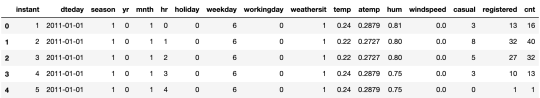
获取每列的数据统计信息:
fullData[number_features].describe()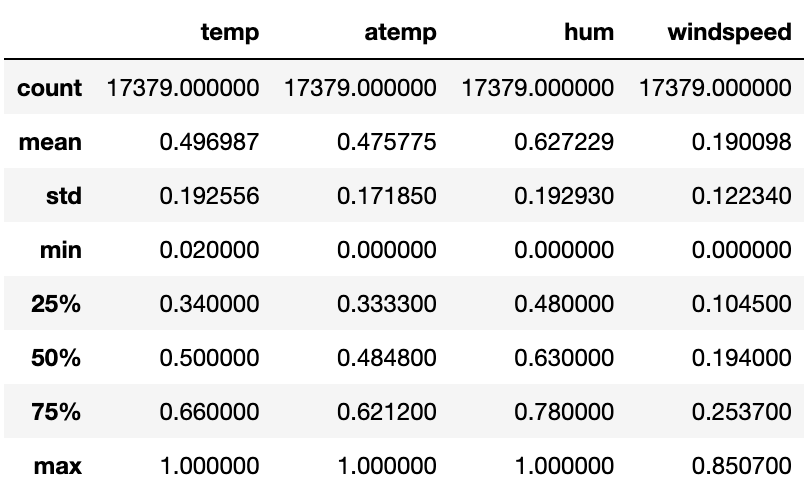
for col in category_features:
    fullData[col] = fullData[col].astype('category')
fullData[category_features].describe()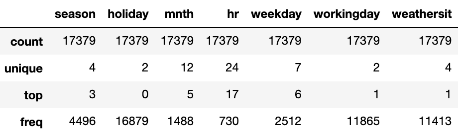
缺失值分析
缺失值分析可参见往期文章:缺失值处理,你真的会了吗?
检查数据中的NULL值:
print(fullData.isnull().any())instant False
dteday False
season False
yr False
mnth False
hr False
holiday False
weekday False
workingday False
weathersit False
temp False
atemp False
hum False
windspeed False
casual False
registered False
cnt False
dtype:bool异常值分析
箱形图
sns.set(font_scale=1.0)
fig, axes = plt.subplots(nrows=3,ncols=2)
fig.set_size_inches(15, 15)
sns.boxplot(data=train,y="cnt",orient="v",ax=axes[0][0])
sns.boxplot(data=train,y="cnt",x="mnth",orient="v",ax=axes[0][1])
sns.boxplot(data=train,y="cnt",x="weathersit",orient="v",ax=axes[1][0])
sns.boxplot(data=train,y="cnt",x="workingday",orient="v",ax=axes[1][1])
sns.boxplot(data=train,y="cnt",x="hr",orient="v",ax=axes[2][0])
sns.boxplot(data=train,y="cnt",x="temp",orient="v",ax=axes[2][1])

axes[0][0].set(ylabel='Count',title="Box Plot On Count")
axes[0][1].set(xlabel='Month', ylabel='Count',title="Box Plot On Count Across Months")
axes[1][0].set(xlabel='Weather Situation', ylabel='Count',title="Box Plot On Count Across Weather Situations")
axes[1][1].set(xlabel='Working Day', ylabel='Count',title="Box Plot On Count Across Working Day")
axes[2][0].set(xlabel='Hour Of The Day', ylabel='Count',title="Box Plot On Count Across Hour Of The Day")
axes[2][1].set(xlabel='Temperature', ylabel='Count',title="Box Plot On Count Across Temperature")

for tick in axes[2][1].get_xticklabels():
    tick.set_rotation(90)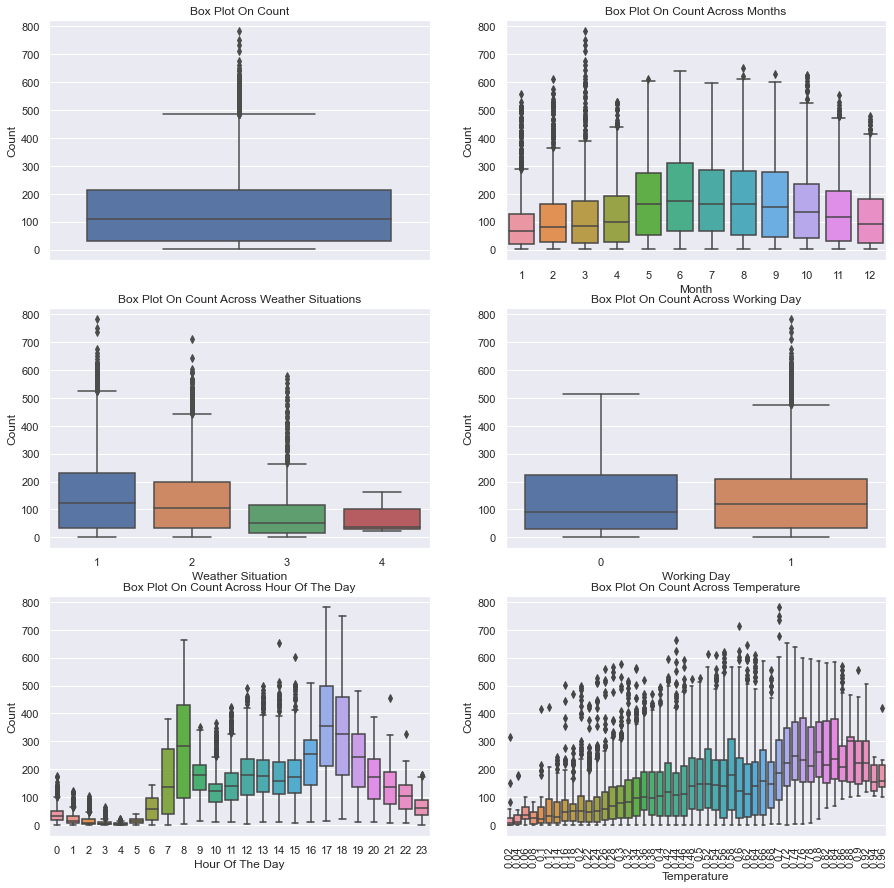
解析: 工作日和节假日箱形图表明,正常工作日出租的自行车比周末或节假日多。每小时的箱形图显示当地早上8点最大,下午5点最大,这表明大多数自行车租赁服务的用户使用自行车上班或上学。另一个重要因素似乎是温度:较高的温度导致自行车租赁数量增加,而较低的温度不仅降低了平均租赁数量,而且在数据中显示出更多的异常值。
从数据中去除异常值
sns.distplot(train[target[-1]]);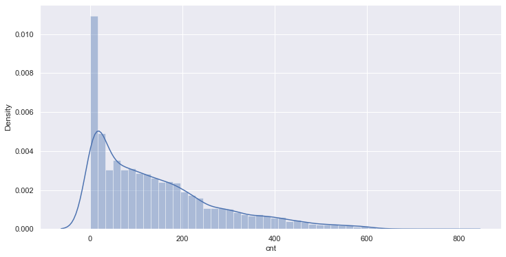
计数值的分布图显示,计数值不符合正态分布。我们将使用中位数和四分位区间(IQR)来识别和去除数据中的异常值。(另一种方法是将目标值转换为正态分布,并使用平均值和标准偏差。)
print("带有异常值的列车集合中的样本: {}".format(len(train)))
q1 = train.cnt.quantile(0.25)
q3 = train.cnt.quantile(0.75)
iqr = q3 - q1
lower_bound = q1 -(1.5 * iqr)
upper_bound = q3 +(1.5 * iqr)
train_preprocessed = train.loc[(train.cnt >= lower_bound) & (train.cnt <= upper_bound)]
print("没有异常值的训练样本集: {}".format(len(train_preprocessed)))
sns.distplot(train_preprocessed.cnt);
带有异常值的列车集合中的样本:10427
没有异常值的训练样本集:10151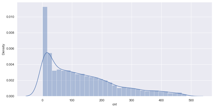
相关分析
matrix = train[number_features + target].corr()
heat = np.array(matrix)
heat[np.tril_indices_from(heat)] = False
fig,ax= plt.subplots()
fig.set_size_inches(15,8)
sns.set(font_scale=1.0)
sns.heatmap(matrix, mask=heat,vmax=1.0, vmin=0.0, square=True,annot=True, cmap="Reds")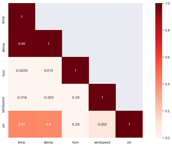
结论: 在描述性分析总结如下几点:
变量"Casual"和"registered"包含关于共享自行车计数直接信息,而如果将这些信息用于预测(数据泄漏)。因此,它们不在特征集中考虑。
变量"temp"和"atemp"是高度相关的。为了降低预测模型的维数,可以删除特征"atemp"。
变量"hr"和"temp"似乎是预测自行车共享数量的贡献较大的特征。
features.remove('atemp')评价指标概述
Mean Squared Error (MSE)
()
Root Mean Squared Logarithmic Error (RMSLE)
(()())
R^2 Score
()
模型选择
所呈现的问题的特点是:
回归:目标变量是一个连续型数值。
数据集小:小于100K的样本量。
少数特征应该是重要的:相关矩阵表明少数特征包含预测目标变量的信息。
这些特点给予了岭回归、支持向量回归、集成回归、随机森林回归等方法大展身手的好机会。有关回归模型可参见往期文章👇。
线性回归中的多重共线性与岭回归
机器学习 | 简单而强大的线性回归详解
机器学习 | 深度理解Lasso回归分析
一文掌握sklearn中的支持向量机
集成算法 | 随机森林回归模型
万字长文,演绎八种线性回归算法最强总结!
原理+代码,总结了 11 种回归模型
机器学习中回归算法的基本数学原理
我们将对这些模型的性能进行如下评估:
x_train = train_preprocessed[features].values
y_train = train_preprocessed[target].values.ravel()
# Sort validation set for plots
val = val.sort_values(by=target)
x_val = val[features].values
y_val = val[target].values.ravel()
x_test = test[features].values

table = PrettyTable()
table.field_names = ["Model",
                     "Mean Squared Error",
                     "R² score"]

models = [
    SGDRegressor(max_iter=1000, tol=1e-3),
    Lasso(alpha=0.1),
    ElasticNet(random_state=0),
    Ridge(alpha=.5),
    SVR(gamma='auto', kernel='linear'),
    SVR(gamma='auto', kernel='rbf'),
    BaggingRegressor(),
    BaggingRegressor(KNeighborsClassifier(),
                     max_samples=0.5,
                     max_features=0.5),
    NuSVR(gamma='auto'),
    RandomForestRegressor(random_state=0,
                          n_estimators=300)
]

for model in models:
    model.fit(x_train, y_train)
    y_res = model.predict(x_val)

    mse = mean_squared_error(y_val, y_res)
    score = model.score(x_val, y_val)

    table.add_row([type(model).__name__,
                  format(mse, '.2f'),
                  format(score, '.2f')])

print(table)
+-----------------------+--------------------+----------+
| Model | Mean Squared Error | R² score |
+-----------------------+--------------------+----------+
| SGDRegressor | 43654.10 | 0.06 |
| Lasso | 43103.36 | 0.07 |
| ElasticNet | 54155.92 | -0.17 |
| Ridge | 42963.88 | 0.07 |
| SVR | 50794.91 | -0.09 |
| SVR | 41659.68 | 0.10 |
| BaggingRegressor | 18959.70 | 0.59 |
| BaggingRegressor | 52475.34 | -0.13 |
| NuSVR | 41517.67 | 0.11 |
| RandomForestRegressor | 18949.93 | 0.59 |
+-----------------------+--------------------+----------+随机森林
随机森林模型
随机森林模型理论和实践可参考如下两篇文章:
集成算法 | 随机森林分类模型
集成算法 | 随机森林回归模型
# Table setup
table = PrettyTable()
table.field_names = ["Model", "Dataset", "MSE", "MAE", 'RMSLE', "R² score"]
# 模型训练
model = RandomForestRegressor(bootstrap=True, criterion='mse', max_depth=None,
           max_features='auto', max_leaf_nodes=None,
           min_impurity_decrease=0.0, min_impurity_split=None,
           min_samples_leaf=1, min_samples_split=4,
           min_weight_fraction_leaf=0.0, n_estimators=200, n_jobs=None,
           oob_score=False, random_state=None, verbose=0, warm_start=False)
model.fit(x_train, y_train)

def evaluate(x, y, dataset):
    pred = model.predict(x)
    mse = mean_squared_error(y, pred)
    mae = mean_absolute_error(y, pred)
    score = model.score(x, y)
    rmsle = np.sqrt(mean_squared_log_error(y, pred))
    table.add_row([type(model).__name__, dataset,
                  format(mse, '.2f'),
                  format(mae, '.2f'),
                  format(rmsle, '.2f'),
                  format(score, '.2f')])

evaluate(x_train, y_train, 'training')
evaluate(x_val, y_val, 'validation')

print(table)
+-----------------------+------------+----------+-------+-------+----------+
| Model | Dataset | MSE | MAE | RMSLE | R² score |
+-----------------------+------------+----------+-------+-------+----------+
| RandomForestRegressor | training | 298.21 | 10.93 | 0.21 | 0.98 |
| RandomForestRegressor | validation | 18967.46 | 96.43 | 0.47 | 0.59 |
+-----------------------+------------+----------+-------+-------+----------+特征重要性
importances = model.feature_importances_
std = np.std([tree.feature_importances_ for tree in model.estimators_], axis=0)
indices = np.argsort(importances)[::-1]
# 打印出特征排序
print("Feature ranking:")
for f in range(x_val.shape[1]):
print("%d. feature %s (%f)" % (f + 1, features[indices[f]], importances[indices[f]]))Feature ranking:
1. feature hr (0.633655)
2. feature temp (0.160043)
3. feature hum (0.049495)
4. feature workingday (0.046797)
5. feature weathersit (0.027105)
6. feature windspeed (0.026471)
7. feature weekday (0.020293)
8. feature mnth (0.019940)
9. feature season (0.012995)
10. feature holiday (0.003206)# 绘制出随机森林的特征重要性
plt.figure(figsize=(14,5))
plt.title("Feature importances")
plt.bar(range(x_val.shape[1]), importances[indices],
color="cornflowerblue", yerr=std[indices], align="center")
plt.xticks(range(x_val.shape[1]), [features[i] for i in indices])
plt.xlim([-1, x_val.shape[1]])
plt.show())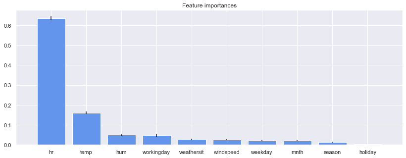
解析: 结果对应于特征相关矩阵中变量"hour"和变量"temperature"与自行车共享计数的高度相关。
写在最后
以下是进一步提高数据模型性能的一些思路:
目标变量的分布调整:有些预测模型假设目标变量的分布为正态分布,在数据预处理中进行转换可以提高这些方法的性能。
大规模数据集随机森林的实现。对于大规模数据集(>10 Mio. 样本),如果不能在工作内存中保存所有的样本,或者会遇到严重的内存问题,那么使用python实现sklearn中的随机森林将会非常慢。一个解决方案可以是woody实现,其中包含用于预分类的顶树,以及在顶树的叶子处用C语言实现的平坦随机森林。

往期精彩回顾


适合初学者入门人工智能的路线及资料下载机器学习及深度学习笔记等资料打印机器学习在线手册深度学习笔记专辑《统计学习方法》的代码复现专辑
AI基础下载黄海广老师《机器学习课程》视频课黄海广老师《机器学习课程》711页完整版课件
本站qq群554839127,加入微信群请扫码:


华为开发者空间,是为全球开发者打造的专属开发空间,汇聚了华为优质开发资源及工具,致力于让每一位开发者拥有一台云主机,基于华为根生态开发、创新。
更多推荐


 11
11 0
0- 0


 已为社区贡献30条内容

所有评论(0)