splines | 多项式回归和样条曲线回归
当变量之间存在非线性关系时,线性回归就不再适用,这时可以转而使用其他非线性模型。但是,线性回归毕竟是统计建模的基础,通过本篇的介绍,可以看到即使是非线性关系有时也可以通过变换然后使用线性回...
当变量之间存在非线性关系时,线性回归就不再适用,这时可以转而使用其他非线性模型。但是,线性回归毕竟是统计建模的基础,通过本篇的介绍,可以看到即使是非线性关系有时也可以通过变换然后使用线性回归进行建模。
1 多项式回归
多项式回归即是在模型中加入自变量的高次幂,如三次多项式回归:
虽然自变量与因变量之间存在着非线性关系,但是以上模型形式仍然可以使用线性回归进行拟合。
体重和身高的关系一般就可以通过三次函数来进行刻画。
model.1 <- lm(weight ~ height,
              data = women)
summary(model.1)
## Coefficients:
##              Estimate Std. Error t value Pr(>|t|)
## (Intercept) -87.51667    5.93694  -14.74 1.71e-09 ***
## height        3.45000    0.09114   37.85 1.09e-14 ***
## ---
## Signif. codes:  0 '***' 0.001 '**' 0.01 '*' 0.05 '.' 0.1 ' ' 1
##
## Residual standard error: 1.525 on 13 degrees of freedom
## Multiple R-squared:  0.991,  Adjusted R-squared:  0.9903
## F-statistic:  1433 on 1 and 13 DF,  p-value: 1.091e-14

model.2 <- lm(weight ~ height + I(height^2) + I(height^3),
              data = women)
summary(model.2)
## Coefficients:
##               Estimate Std. Error t value Pr(>|t|)
## (Intercept) -8.967e+02  2.946e+02  -3.044  0.01116 *
## height       4.641e+01  1.366e+01   3.399  0.00594 **
## I(height^2) -7.462e-01  2.105e-01  -3.544  0.00460 **
## I(height^3)  4.253e-03  1.079e-03   3.940  0.00231 **
## ---
## Signif. codes:  0 '***' 0.001 '**' 0.01 '*' 0.05 '.' 0.1 ' ' 1
##
## Residual standard error: 0.2583 on 11 degrees of freedom
## Multiple R-squared:  0.9998, Adjusted R-squared:  0.9997
## F-statistic: 1.679e+04 on 3 and 11 DF,  p-value: < 2.2e-16
从调整R方的角度看,线性模型就能很好地拟合二者的关系,但是三次多项式回归的拟合优度更高。
plot(women$height, women$weight, type = "p",
     xlab = "drat", ylab = "mpg", family = "mono")
lines(women$height, fitted(model.1), col = "blue")
lines(women$height, fitted(model.2), col = "red")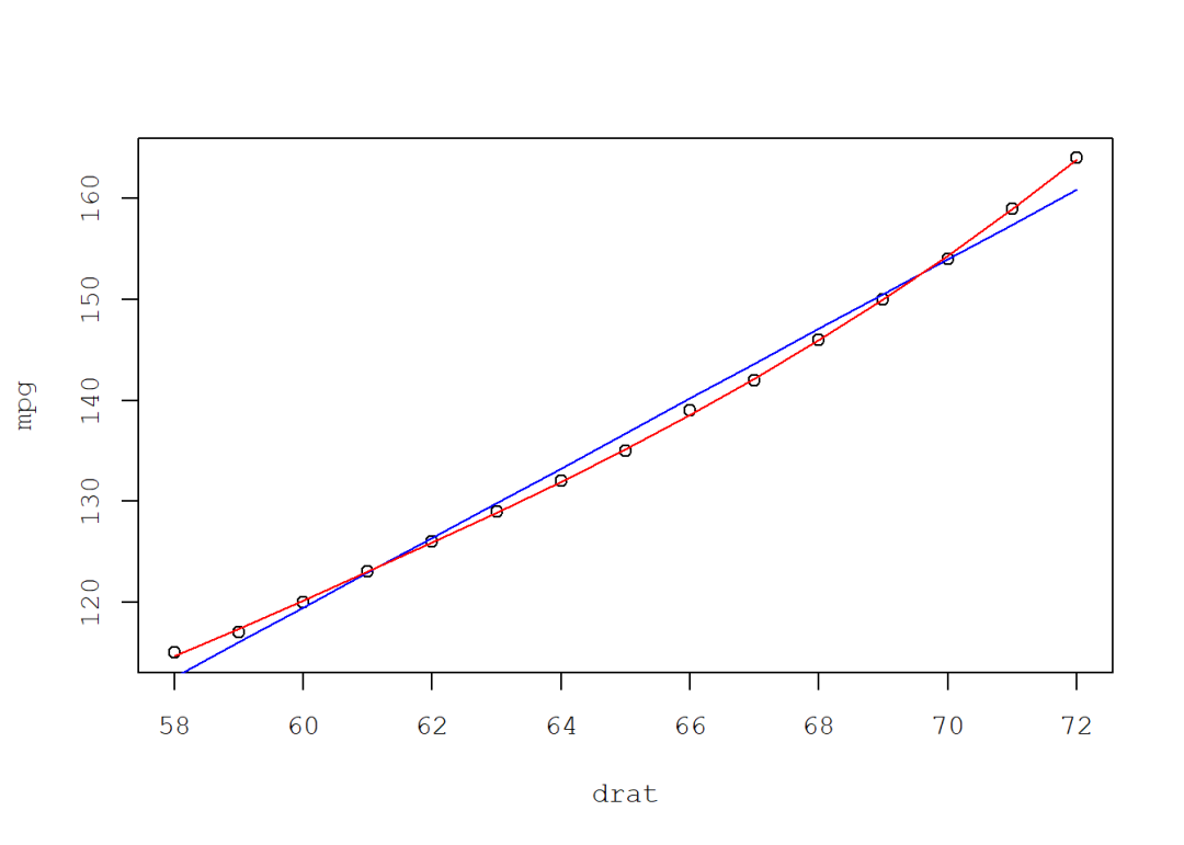
从图中也可以看出,三次多项式回归对样本的拟合度更高。
多项式回归更优雅的写法是使用poly()函数,它的语法结构如下:
poly(x, ..., degree = 1, coefs = NULL, raw = FALSE, simple = FALSE)
x:自变量;
degree:多项式回归的最高次幂。
使用该函数生成的是一个基矩阵(basis matrix),其行数与样本数相同,列数与自由度相同,也即多项式的最高次幂。
poly(women$height, degree = 3)
##                   1           2             3
##  [1,] -4.183300e-01  0.47227028 -4.562564e-01
##  [2,] -3.585686e-01  0.26986873 -6.517949e-02
##  [3,] -2.988072e-01  0.09860588  1.754832e-01
##  [4,] -2.390457e-01 -0.04151827  2.908008e-01
##  [5,] -1.792843e-01 -0.15050372  3.058422e-01
##  [6,] -1.195229e-01 -0.22835046  2.456765e-01
##  [7,] -5.976143e-02 -0.27505851  1.353728e-01
##  [8,]  1.326970e-17 -0.29062786 -4.453155e-17
##  [9,]  5.976143e-02 -0.27505851 -1.353728e-01
## [10,]  1.195229e-01 -0.22835046 -2.456765e-01
## [11,]  1.792843e-01 -0.15050372 -3.058422e-01
## [12,]  2.390457e-01 -0.04151827 -2.908008e-01
## [13,]  2.988072e-01  0.09860588 -1.754832e-01
## [14,]  3.585686e-01  0.26986873  6.517949e-02
## [15,]  4.183300e-01  0.47227028  4.562564e-01
## attr(,"coefs")
## attr(,"coefs")$alpha
## [1] 65 65 65
##
## attr(,"coefs")$norm2
## [1]     1.000    15.000   280.000  4125.333 57283.200
##
## attr(,"degree")
## [1] 1 2 3
## attr(,"class")
## [1] "poly"   "matrix"
基矩阵的每一列相当于一个新的变量,将生成的基矩阵放入线性模型表达式中,相当于拟合因变量与这些新变量之间的线性关系。
model.3 <- lm(weight ~ poly(height, 3),
              data = women)
summary(model.3)
## Coefficients:
##                  Estimate Std. Error t value Pr(>|t|)
## (Intercept)      136.7333     0.0667 2049.86  < 2e-16 ***
## poly(height, 3)1  57.7295     0.2583  223.46  < 2e-16 ***
## poly(height, 3)2   5.3351     0.2583   20.65 3.79e-10 ***
## poly(height, 3)3   1.0178     0.2583    3.94  0.00231 **
## ---
## Signif. codes:  0 '***' 0.001 '**' 0.01 '*' 0.05 '.' 0.1 ' ' 1
##
## Residual standard error: 0.2583 on 11 degrees of freedom
## Multiple R-squared:  0.9998, Adjusted R-squared:  0.9997
## F-statistic: 1.679e+04 on 3 and 11 DF,  p-value: < 2.2e-16

plot(women$height, women$weight, type = "p",
     xlab = "drat", ylab = "mpg", family = "mono")
lines(women$height, fitted(model.2), col = "red", lty = 3)
lines(women$height, fitted(model.3), col = "blue", lty = 2)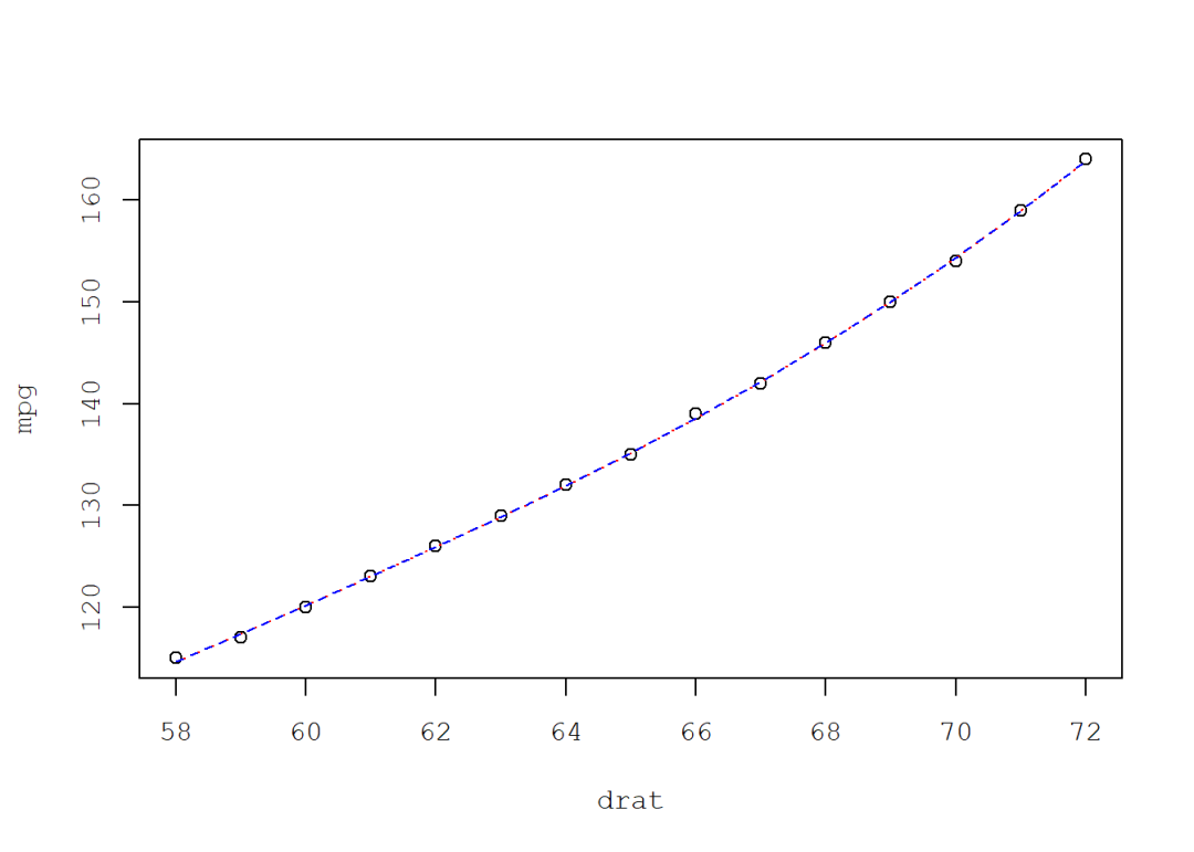
通过上图可以看出,
model.2和model.3实质是相同的。
2 样条曲线回归
样条曲线回归是使用多段平滑曲线对样本数据进行拟合,并保证这些曲线的接口处也是平滑的,即两侧曲线在接口处的拟合值和导数均一致。常用的平滑曲线有B样条曲线和自然样条曲线。
2.1 B样条曲线
B样条曲线是由若干个最高幂相同的多项式曲线组成的。在R语言中,可以使用splines工具包中的bs()函数来获得B样条曲线的基矩阵。该函数的语法结构如下:
bs(x, df = NULL, knots = NULL, degree = 3, intercept = FALSE,
   Boundary.knots = range(x))
B样条曲线的主要参数有:
degree:多项式的最高次幂;默认取3;
knots:曲线分段的节点位置,默认为NULL;
intercept:截距;默认不包含截距;
df:自由度;在无截距时,等于最高次幂与节点个数之和,有截距时再加上1。
与poly()函数一样,ns()生成的也是列数与自由度相等的基矩阵。
library(splines)
bs(women$height, knots = c(60, 66), intercept = T)
##           1           2            3           4           5          6
##  [1,] 1.000 0.000000000 0.0000000000 0.000000000 0.000000000 0.00000000
##  [2,] 0.125 0.726562500 0.1439732143 0.004464286 0.000000000 0.00000000
##  [3,] 0.000 0.562500000 0.4017857143 0.035714286 0.000000000 0.00000000
##  [4,] 0.000 0.325520833 0.5608878968 0.112433862 0.001157407 0.00000000
##  [5,] 0.000 0.166666667 0.6031746032 0.220899471 0.009259259 0.00000000
##  [6,] 0.000 0.070312500 0.5591517857 0.339285714 0.031250000 0.00000000
##  [7,] 0.000 0.020833333 0.4593253968 0.445767196 0.074074074 0.00000000
##  [8,] 0.000 0.002604167 0.3342013889 0.518518519 0.144675926 0.00000000
##  [9,] 0.000 0.000000000 0.2142857143 0.535714286 0.250000000 0.00000000
## [10,] 0.000 0.000000000 0.1240079365 0.483630952 0.387731481 0.00462963
## [11,] 0.000 0.000000000 0.0634920635 0.380952381 0.518518519 0.03703704
## [12,] 0.000 0.000000000 0.0267857143 0.254464286 0.593750000 0.12500000
## [13,] 0.000 0.000000000 0.0079365079 0.130952381 0.564814815 0.29629630
## [14,] 0.000 0.000000000 0.0009920635 0.037202381 0.383101852 0.57870370
## [15,] 0.000 0.000000000 0.0000000000 0.000000000 0.000000000 1.00000000
## attr(,"degree")
## [1] 3
## attr(,"knots")
## [1] 60 66
## attr(,"Boundary.knots")
## [1] 58 72
## attr(,"intercept")
## [1] TRUE
## attr(,"class")
## [1] "bs"     "basis"  "matrix"
因为
degree默认值等于3,又节点数等于2且包含截距,因此自由度为6。
默认情况下,ns()函数放到线性模型表达式中实现的三次多项式回归的效果:
model.4 <- lm(weight ~ bs(height),
              data = women)
summary(model.4)

plot(women$height, women$weight, type = "p",
     xlab = "drat", ylab = "mpg", family = "mono")
lines(women$height, fitted(model.3), col = "red", lty = 3)
lines(women$height, fitted(model.4), col = "blue", lty = 2)
样条曲线回归和多项式回归的差别就在于,它可以通过增加自由度或节点来实现分段回归并保持接口处平滑。一般情况下,样条曲线使用的都是三次样条,即degree = 3。下面代码比较了自由度分别为5、6、7时的B样条曲线回归结果:
model.5 <- lm(mpg ~ bs(drat, df = 5), data = mtcars)
model.6 <- lm(mpg ~ bs(drat, df = 6), data = mtcars)
model.7 <- lm(mpg ~ bs(drat, df = 7), data = mtcars)

simdata <- data.frame(drat = seq(1,5,0.001))
plot(mtcars$drat, mtcars$mpg, type = "p",
     xlab = "drat", ylab = "mpg", family = "mono")
lines(simdata$drat, predict(model.5, simdata), col = "red")
lines(simdata$drat, predict(model.6, simdata), col = "lightblue")
lines(simdata$drat, predict(model.7, simdata), col = "brown")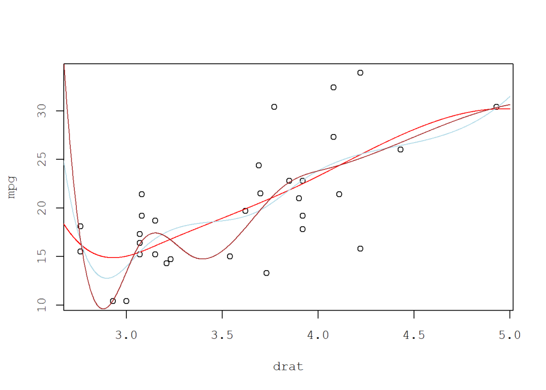
2.2 自然样条曲线
自然样条曲线是一个带有约束条件的三次样条曲线。在R语言中,可以通过splines工具包中的ns()函数生成它的基矩阵。该函数语法结构如下:
ns(x, df = NULL, knots = NULL, intercept = FALSE,
   Boundary.knots = range(x))
自然样条曲线的
degree恒为3,因此函数中不需要有degree参数。
model.8 <- lm(mpg ~ ns(drat, df = 5), data = mtcars)
model.9 <- lm(mpg ~ ns(drat, df = 6), data = mtcars)
model.10 <- lm(mpg ~ ns(drat, df = 7), data = mtcars)

simdata <- data.frame(drat = seq(1,5,0.001))
plot(mtcars$drat, mtcars$mpg, type = "p",
     xlab = "drat", ylab = "mpg", family = "mono")
lines(simdata$drat, predict(model.5, simdata), col = "red")
lines(simdata$drat, predict(model.6, simdata), col = "lightblue")
lines(simdata$drat, predict(model.7, simdata), col = "brown")
lines(simdata$drat, predict(model.8, simdata), col = "red", lty = 2)
lines(simdata$drat, predict(model.9, simdata), col = "lightblue", lty = 2)
lines(simdata$drat, predict(model.10, simdata), col = "brown", lty = 2)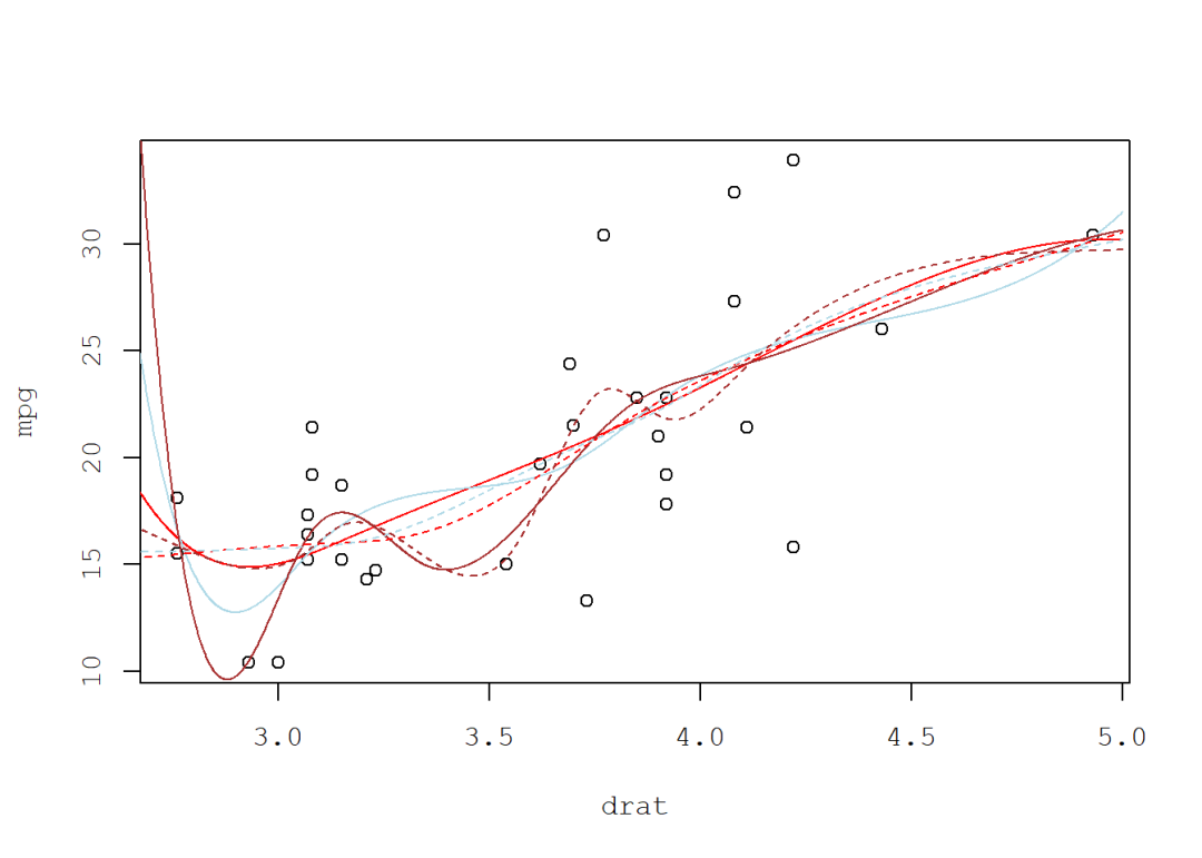

为开发者提供学习成长、分享交流、生态实践、资源工具等服务,帮助开发者快速成长。
更多推荐


 6
6 0
0- 0


 已为社区贡献10条内容

所有评论(0)