【Matplotlib】matplotlib.animation.FuncAnimation绘制动态图、交互式绘图汇总（附官方文档）

文章目录一、以sin举例，motplotlib绘制动图1、绘制sin函数2、动态画出sin函数曲线3、点在曲线上运动4、点，坐标运动二、单摆例子三、滚动的球的例子四、动态条形图五、动态折线图六、交互式绘图七、交互式绘图、混淆矩阵可视化参考一、以sin举例，motplotlib绘制动图1、绘制sin函数import numpy as npimport matplotlibimport matplot

miracleo_

9605人浏览 · 2021-04-02 22:25:16

miracleo_ · 2021-04-02 22:25:16 发布

零、文中用到的相关知识：

函数FuncAnimation

函数FuncAnimation(fig,func,frames,init_func,interval,blit)是绘制动图的主要函数，其参数如下：
    a.fig 绘制动图的画布名称`
    b.func自定义动画函数，即下边程序定义的函数update
    c.frames动画长度，一次循环包含的帧数，在函数运行时，其值会传递给函数update(n)的形参“n”
    d.init_func自定义开始帧，即传入刚定义的函数init,初始化函数
    e.interval更新频率，以ms计
    f.blit选择更新所有点，还是仅更新产生变化的点。应选择True，但mac用户请选择False，否则无法显

plt画布调整函数

# 调整画布里图像的位置
plt.subplots_adjust(top=0.88,
				bottom=0.11,
				left=0.11,
				right=0.9,
				hspace=0.2,
				wspace=0.2)
# 使图像在画布上尽可能大，贴着画布边缘
plt.tight_layout()
# 设置画布尺寸
plt.figure(figsize=(11, 5.6))

说在前面，本文介绍了matplotlib两种绘图方式
- plot.pause
- animation

一、以sin举例，motplotlib绘制动图

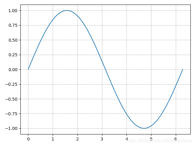
1、绘制sin函数

# # 在绘制动画前，我们需将其sin函数的背景绘制出来。

x = np.linspace(0, 2 * np.pi, 100)
y = np.sin(x)
# tight_layout 调整子图之间及其周围的填充。
fig = plt.figure(tight_layout=True)
plt.plot(x, y)
plt.grid(ls="--")
plt.savefig("sin_test1.png")
plt.show()

在这里插入图片描述

2、动态画出sin函数曲线

# 动态画出sin函数曲线
import numpy as np
import matplotlib.pyplot as plt
from matplotlib.animation import FuncAnimation

# 生成子图，相当于fig = plt.figure(),ax = fig.add_subplot(),其中ax的函数参数表示把当前画布进行分割，
fig, ax = plt.subplots()
xdata, ydata = [], []
ln, = ax.plot([], [], 'r-', animated=False)


def init():
    ax.set_xlim(0, 2 * np.pi)
    ax.set_ylim(-1, 1)
    # 返回曲线
    return ln,


def update(frame):
    # 将每次传过来的n追加到xdata中
    xdata.append(frame)
    ydata.append(np.sin(frame))
    # 重新设置曲线的值
    ln.set_data(xdata, ydata)
    return ln,

'''
函数FuncAnimation(fig,func,frames,init_func,interval,blit)是绘制动图的主要函数，其参数如下：
    a.fig 绘制动图的画布名称
    b.func自定义动画函数，即下边程序定义的函数update
    c.frames动画长度，一次循环包含的帧数，在函数运行时，其值会传递给函数update(n)的形参“n”
    d.init_func自定义开始帧，即传入刚定义的函数init,初始化函数
    e.interval更新频率，以ms计
    f.blit选择更新所有点，还是仅更新产生变化的点。应选择True，但mac用户请选择False，否则无法显
'''
ani = FuncAnimation(fig=fig, func=update, frames=np.linspace(0, 2 * np.pi, 128),
                    init_func=init, blit=True)

plt.show()

ani.save('sin_test1.gif', writer='imagemagick', fps=100)

在这里插入图片描述

3、点在曲线上运动

import numpy as np
import matplotlib
import matplotlib.pyplot as plt
import matplotlib.animation as animation


# 首先定义了一个update_points函数，用于更新绘制的图中的数据点。此函数的输入参数num代表当前动画的第几帧，
# 函数的返回，即为我们需要更新的对象，需要特别注意的是：reuturn point_ani,这个逗号一定加上，否则动画不能
# 正常显示。当然这里面操作的点对象point_ani我们一般会提前声明得到：point_ani, = plt.plot(x[0], y[0], "ro")。
# 接下来就是将此函数传入我们的FuncAnimation函数中，函数的参数说明可以参见官网，这里简要说明用到的几个参数。
# 第1个参数fig：即为我们的绘图对象.
# 第2个参数update_points：更新动画的函数.
# 第3个参数np.arrange(0, 100)：动画帧数，这需要是一个可迭代的对象。
# interval参数：动画的时间间隔。
# blit参数：是否开启某种动画的渲染。

def update_points(num):
    '''
    更新数据点
    '''
    point_ani.set_data(x[num], y[num])
    return point_ani,


x = np.linspace(0, 2 * np.pi, 100)
y = np.sin(x)

fig = plt.figure(tight_layout=True)
plt.plot(x, y)
point_ani, = plt.plot(x[0], y[0], "ro")
plt.grid(ls="--")
# 开始制作动画
ani = animation.FuncAnimation(fig, update_points, np.arange(0, 100), interval=100, blit=True)

ani.save('sin_test2.gif', writer='imagemagick', fps=10)
plt.show()

在这里插入图片描述

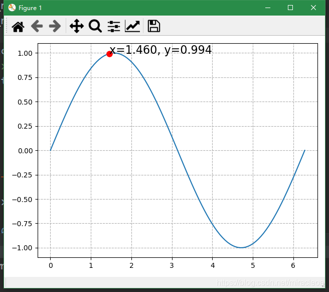
4、点，坐标运动

import numpy as np
import matplotlib
import matplotlib.pyplot as plt
import matplotlib.animation as animation


# 我们可以往其中添加一些文本显示，或者在不同的条件下改变点样式。这其实也非常简单，
# 只需在update_points函数中添加一些额外的，你想要的效果代码即可。
# 我在上面update_points函数中添加了一个文本，让它显示点的(x, y)的坐标值，
# 同时在不同的帧，改变了点的形状，让它在5的倍数帧显示为五角星形状。

# def update_points(num):
#     if num % 5 == 0:
#         point_ani.set_marker("*")
#         point_ani.set_markersize(12)
#     else:
#         point_ani.set_marker("o")
#         point_ani.set_markersize(8)
#
#     point_ani.set_data(x[num], y[num])
#     text_pt.set_text("x=%.3f, y=%.3f" % (x[num], y[num]))
#     return point_ani, text_pt,


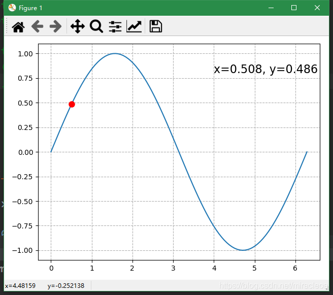
# 再稍微改变一下，可以让文本跟着点动。只需将上面的代码update_points函数改为如下代码，其效果如图2-4所示。
def update_points(num):
    point_ani.set_data(x[num], y[num])
    if num % 5 == 0:
        point_ani.set_marker("*")
        point_ani.set_markersize(12)
    else:
        point_ani.set_marker("o")
        point_ani.set_markersize(8)

    text_pt.set_position((x[num], y[num]))
    text_pt.set_text("x=%.3f, y=%.3f" % (x[num], y[num]))
    return point_ani, text_pt,


x = np.linspace(0, 2 * np.pi, 100)
y = np.sin(x)

fig = plt.figure(tight_layout=True)
plt.plot(x, y)
point_ani, = plt.plot(x[0], y[0], "ro")
plt.grid(ls="--")
text_pt = plt.text(4, 0.8, '', fontsize=16)

ani = animation.FuncAnimation(fig, update_points, np.arange(0, 100), interval=100, blit=True)

ani.save('sin_test3.gif', writer='imagemagick', fps=10)
plt.show()

（1）上述代码，第一个函数
（2）上述代码，第二个函数

二、单摆例子

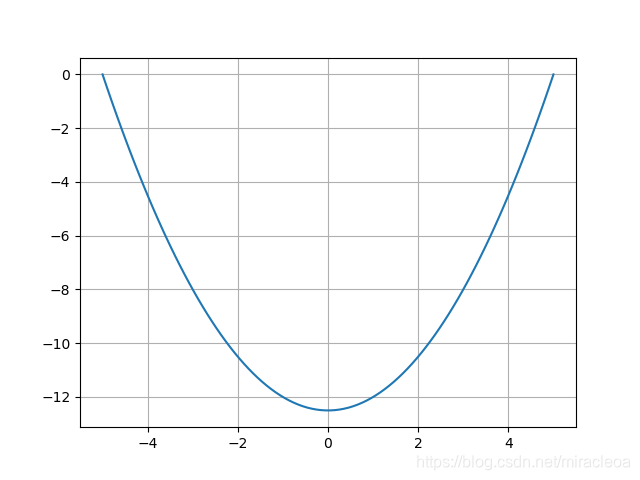
1、scipy中odeint函数用法

odeint()函数是scipy库中一个数值求解微分方程的函数
odeint()函数需要至少三个变量，第一个是微分方程函数，第二个是微分方程初值，第三个是微分的自变量。
一个一阶微分方程例子

import numpy as np
import matplotlib.pyplot as plt
from scipy.integrate import odeint


def diff(y, x):
    return np.array(x)


# 上面定义的函数在odeint里面体现的就是dy/dx = x
x = np.linspace(-5, 5, 100)  # 给出x范围
y = odeint(diff, 0, x)  # 设初值为0 此时y为一个数组，元素为不同x对应的y值
# 也可以直接y = odeint(lambda y, x: x, 0, x)
plt.plot(x, y[:, 0])  # y数组（矩阵）的第一列，（因为维度相同，plt.plot(x, y)效果相同）
plt.grid()
plt.savefig("odeint.png")
plt.show()

在这里插入图片描述

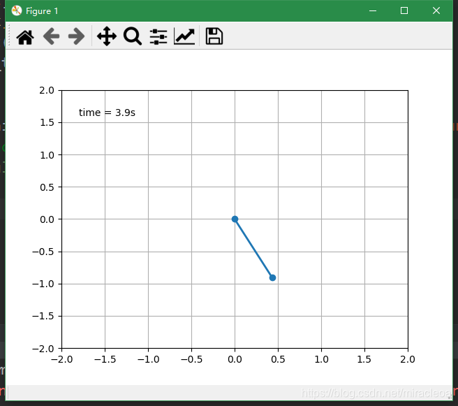
2、单摆例子

# -*- coding: utf-8 -*-

from math import sin, cos
import numpy as np
from scipy.integrate import odeint
import matplotlib.pyplot as plt
import matplotlib.animation as animation

g = 9.8
leng = 1.0
b_const = 0.2

# no decay case:
def pendulum_equations1(w, t, l):
    th, v = w
    dth = v
    dv  = - g/l * sin(th)
    return dth, dv

# the decay exist case:
def pendulum_equations2(w, t, l, b):
    th, v = w
    dth = v
    dv = -b/l * v - g/l * sin(th)
    return dth, dv

t = np.arange(0, 20, 0.1)
track = odeint(pendulum_equations1, (1.0, 0), t, args=(leng,))
#track = odeint(pendulum_equations2, (1.0, 0), t, args=(leng, b_const))
xdata = [leng*sin(track[i, 0]) for i in range(len(track))]
ydata = [-leng*cos(track[i, 0]) for i in range(len(track))]

fig, ax = plt.subplots()
ax.grid()
line, = ax.plot([], [], 'o-', lw=2)
time_template = 'time = %.1fs'
time_text = ax.text(0.05, 0.9, '', transform=ax.transAxes)

def init():
    ax.set_xlim(-2, 2)
    ax.set_ylim(-2, 2)
    time_text.set_text('')
    return line, time_text

def update(i):
    newx = [0, xdata[i]]
    newy = [0, ydata[i]]
    line.set_data(newx, newy)
    time_text.set_text(time_template %(0.1*i))
    return line, time_text

ani = animation.FuncAnimation(fig, update, range(1, len(xdata)), init_func=init, interval=50)
#ani.save('single_pendulum_decay.gif', writer='imagemagick', fps=100)
ani.save('single_pendulum_nodecay.gif', writer='imagemagick', fps=100)
plt.show()

在这里插入图片描述

三、滚动的球的例子

import numpy as np 
import matplotlib.pyplot as plt 
import matplotlib.animation as animation

fig = plt.figure(figsize=(6, 6))
ax = plt.gca()
ax.grid()
ln1, = ax.plot([], [], '-', lw=2)
ln2, = ax.plot([], [], '-', color='r', lw=2)
theta = np.linspace(0, 2*np.pi, 100)
r_out = 1
r_in = 0.5

def init():
    ax.set_xlim(-2, 2)
    ax.set_ylim(-2, 2)
    x_out = [r_out*np.cos(theta[i]) for i in range(len(theta))]
    y_out = [r_out*np.sin(theta[i]) for i in range(len(theta))]
    ln1.set_data(x_out, y_out)
    return ln1,

def update(i):
    x_in = [(r_out-r_in)*np.cos(theta[i])+r_in*np.cos(theta[j]) for j in range(len(theta))]
    y_in = [(r_out-r_in)*np.sin(theta[i])+r_in*np.sin(theta[j]) for j in range(len(theta))]
    ln2.set_data(x_in, y_in)
    return ln2,

ani = animation.FuncAnimation(fig, update, range(len(theta)), init_func=init, interval=30)
ani.save('roll.gif', writer='imagemagick', fps=100)

plt.show()

在这里插入图片描述

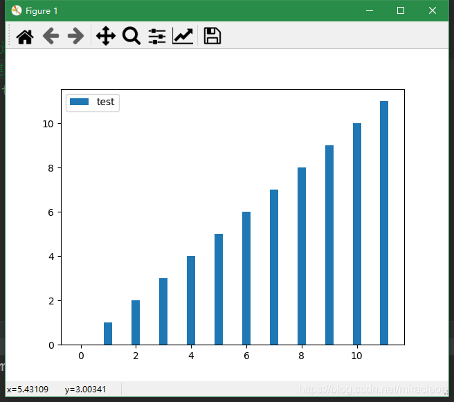
四、动态条形图

动态条形图
基本原理是将数据放入数组，然后每次往数组里面增加一个数，清除之前的图，重新画出图像。

import matplotlib.pyplot as plt
fig, ax = plt.subplots()
y1 = []
for i in range(50):
    y1.append(i)  # 每迭代一次，将i放入y1中画出来
    ax.cla()   # 清除键
    ax.bar(y1, label='test', height=y1, width=0.3)
    ax.legend()
    plt.pause(0.1)

在这里插入图片描述

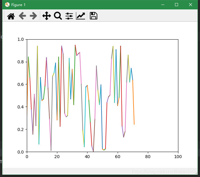
五、动态折线图

import numpy as np
import matplotlib.pyplot as plt

plt.axis([0, 100, 0, 1])
plt.ion()

xs = [0, 0]
ys = [1, 1]

for i in range(100):
    y = np.random.random()
    xs[0] = xs[1]
    ys[0] = ys[1]
    xs[1] = i
    ys[1] = y
    plt.plot(xs, ys)
    plt.pause(0.1)

在这里插入图片描述

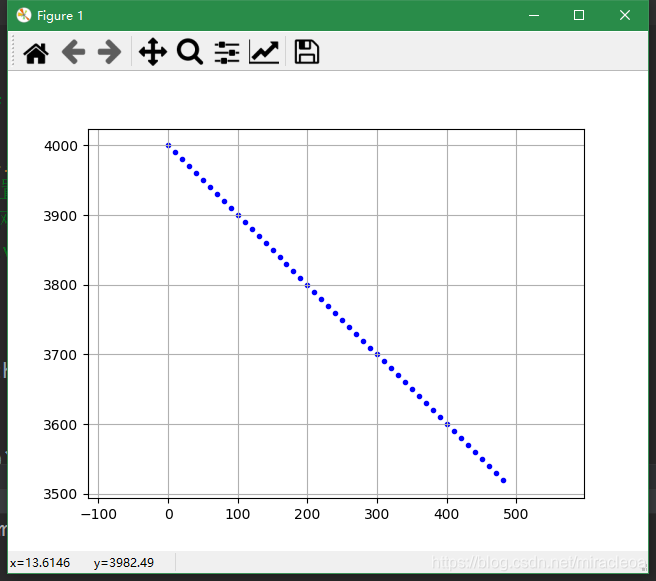
六、交互式绘图

绘图语句中加入pl.ion()时，表示打开了交互模式。此时python解释器解释完所有命令后，给你出张图，但不会结束会话，而是等着你跟他交流交流。如果你继续往代码中加入语句，run之后，你会实时看到图形的改变。当绘图语句中加入pl.ioff()时或不添加pl.ion()时，表示打关了交互模式。此时要在代码末尾加入pl.show()才能显示图片。python解释器解释完所有命令后，给你出张图，同时结束会话。如果你继续往代码中加入语句，再不会起作用，除非你关闭当前图片，重新run。

# -*- coding: utf-8 -*-

import matplotlib.pyplot as plt
from matplotlib.patches import Circle
import numpy as np
import math

plt.close()  # clf() # 清图 cla() # 清坐标轴 close() # 关窗口
fig = plt.figure()
ax = fig.add_subplot(1, 1, 1)
ax.axis("equal")  # 设置图像显示的时候XY轴比例
plt.grid(True)  # 添加网格
plt.ion()  # interactive mode on
IniObsX = 0000
IniObsY = 4000
IniObsAngle = 135
IniObsSpeed = 10 * math.sqrt(2)  # 米/秒
print('开始仿真')
try:
    for t in range(180):
        # 障碍物船只轨迹
        obsX = IniObsX + IniObsSpeed * math.sin(IniObsAngle / 180 * math.pi) * t
        obsY = IniObsY + IniObsSpeed * math.cos(IniObsAngle / 180 * math.pi) * t
        ax.scatter(obsX, obsY, c='b', marker='.')  # 散点图
        # ax.lines.pop(1) 删除轨迹
        # 下面的图,两船的距离
        plt.pause(0.001)
except Exception as err:
    print(err)

在这里插入图片描述

七、交互式绘图、混淆矩阵可视化

import numpy as np
import matplotlib.pyplot as plt
from matplotlib.widgets import Slider

omega = 1.0
x = np.arange(1000) / 200
y = np.sin(omega * x)

F = plt.figure()  # 创建一个Figure
axes_for_plot = F.add_axes([0.2, 0.2, 0.6, 0.6])  # 增加一个Axes，用于绘图
plot_object, = axes_for_plot.plot(x, y)  # 在这个Axes上绘图


def slider_event(event):
    new_omega = slider_object.val  # 获取控件值
    new_y = np.sin(new_omega * x)  # 计算更新后的数据
    plot_object.set_ydata(new_y)  # 利用新数据更新已有的图


axes_for_slider = F.add_axes([0.2, 0.05, 0.6, 0.05])  # 增加一个Axes，放置滑块
slider_object = Slider(label='omega',
                       valmin=0.1, valmax=2, valinit=1.0,
                       ax=axes_for_slider)
slider_object.on_changed(slider_event)  # 为滑块绑定方法

plt.show()