1.题目

试使用LIBSVM，在西瓜数据集3.0α上分别用线性核和高斯核训练一个SVM，并比较其支持向量的差别。

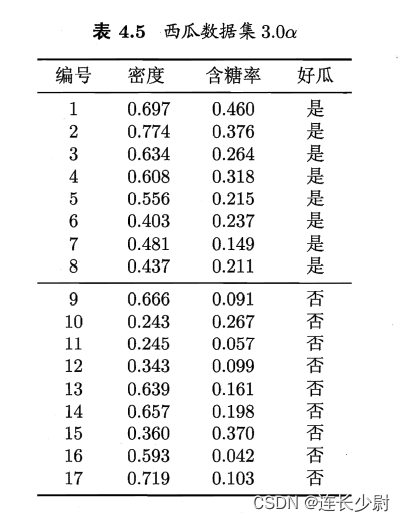
西瓜数据集3.0α如下图：

2.LIBSVM

libsvm是目前比较著名的SVM软件包，由台湾大学林智仁(Chih-Jen Lin)教授等开发，它可以帮助程序员轻松的实现SVM二分类、多分类或者SVR等任务。
LIBSVM官网：https://www.csie.ntu.edu.tw/~cjlin/libsvm/

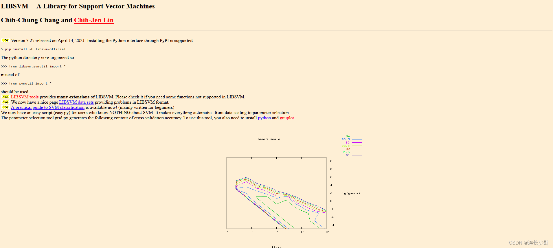
可以根据官网新手引导进行下载和配置，这里就直接使用anaconda进行安装了。
在anaconda控制台中输入

pip install libsvm

即可安装。

3. 代码实现

因为我过去下载的数据集是xlsx格式，所以这里需要将表格数据转成libsvm要求的数据格式。当然，下面我将转换完的数据放进来了，如果需要可以直接复制粘贴。
libsvm要求数据集为以下格式：数据集包含若干行，每行对应一个样例，对于每个样例有以下格式：

[类别] [属性编号1]:[属性值1] [属性编号2]:[属性值2] …

以本题的西瓜数据为例子，转换完就是这样：

1 1:0.697 2:0.46
1 1:0.774 2:0.376
1 1:0.634 2:0.264
1 1:0.608 2:0.318
1 1:0.556 2:0.215
1 1:0.403 2:0.237
1 1:0.481 2:0.149
1 1:0.437 2:0.211
0 1:0.666 2:0.091
0 1:0.243 2:0.267
0 1:0.245 2:0.057
0 1:0.343 2:0.099
0 1:0.639 2:0.161
0 1:0.657 2:0.198
0 1:0.36 2:0.37
0 1:0.593 2:0.042
0 1:0.719 2:0.103

对于第一行： ”1 1:0.697 2:0.46“，
从左到右数字依次的含义是，“1” 表示第1个类别，“1:0.697” 表示第一个属性取值0.697，“2:0.46” 表示第二个属性取值0.46。
然后，将上述格式的数据存在一个.scale或者.txt文件，就可作为libsvm的训练数据，留给后续步骤使用。

from libsvm.svm import *
from libsvm.svmutil import *
import openpyxl
import matplotlib as mpl
import matplotlib.pyplot as plt
import numpy as np

def xl_to_scale_file():
    workbook = openpyxl.load_workbook("../第三章_线性模型/xigua3.0.xlsx")
    sheet1 = workbook['Sheet1']
    with open("./xigua.scale", 'w') as f:
        i = 0
        data_class = sheet1[3][i]
        
        for i in range(sheet1.max_column):
            data_class = sheet1[3][i]
            atr_1 = sheet1[1][i]
            atr_2 = sheet1[2][i]
            line = str(data_class.value) + " 1:" + str(atr_1.value) + " 2:" + str(atr_2.value)
            f.writelines(line + "\n")

然后，就可以调用libsvm了。
首先使用 svm_read_problem() 将训练集读入进来：

train_label, train_value = svm_read_problem("./xigua.scale")

然后，调用svm_train()训练svm，第一个参数为训练标签，第二个数据为训练样本，第三个数据为字符串，用来指定svm的参数，其可以指定的参数完整版说明如下：

options:
-s svm_type : set type of SVM (default 0)
0 – C-SVC
1 – nu-SVC
2 – one-class SVM
3 – epsilon-SVR
4 – nu-SVR
-t kernel_type : set type of kernel function (default 2)
0 – linear: u’v
1 – polynomial: (gammau’v + coef0)^degree
2 – radial basis function: exp(-gamma|u-v|^2)
3 – sigmoid: tanh(gamma*u’v + coef0)
-d degree : set degree in kernel function (default 3)
-g gamma : set gamma in kernel function (default 1/num_features)
-r coef0 : set coef0 in kernel function (default 0)
-c cost : set the parameter C of C-SVC, epsilon-SVR, and nu-SVR (default 1)
-n nu : set the parameter nu of nu-SVC, one-class SVM, and nu-SVR (default 0.5)
-p epsilon : set the epsilon in loss function of epsilon-SVR (default 0.1)
-m cachesize : set cache memory size in MB (default 100)
-e epsilon : set tolerance of termination criterion (default 0.001)
-h shrinking: whether to use the shrinking heuristics, 0 or 1 (default 1)
-b probability_estimates: whether to train a SVC or SVR model for probability estimates, 0 or 1 (default 0)
-wi weight: set the parameter C of class i to weightC, for C-SVC (default 1)

这里只用到其中两个：
-t 用于指定核函数，
0——线性核
2——高斯核
-c 用于指定C-SVC（经典SVM分类）优化目标函数中的参数C，可以理解为代价，当代价越高时，表示对于分类出错的代价越高，SVM的优化过程如下式。其中 ${\xi }_i$ 是松弛变量，表示第i个样例分类错误的程度（比如，如果一个正例被分到了反例那边，它距离超平面越远，则${\xi }_i$越大）
$$\underset{w,b,\xi }{\min }\frac{1}{2}{w}^{T}w+C\sum _l^{i=1}{\xi }_i$$
这里先设置核函数为线性核，c为100

model = svm_train(train_label, train_value, '-t 0 -c 100')

然后，计算准确率：

p_label, p_acc, p_val = svm_predict(train_label, train_value, model)

然后，为了可以展示效果，可以对其进行可视化，代码如下：

train_label, train_value = svm_read_problem("./xigua.scale")
x1 = [mapi[1] for mapi in train_value]
x2 = [mapi[2] for mapi in train_value]
x = np.c_[x1,x2]

np_x = np.asarray(x)
np_y = np.asarray(train_label)
N, M = 100, 100

x1_min, x2_min = np_x.min(axis=0)
x1_max, x2_max = np_x.max(axis=0)

x1_min -= 0.1
x2_min -= 0.1
x1_max += 0.1 
x2_max += 0.1

t1 = np.linspace(x1_min, x1_max, N)
t2 = np.linspace(x2_min, x2_max, M)

grid_x, grid_y = np.meshgrid(t1,t2)

grid = np.stack([grid_x.flat, grid_y.flat], axis=1)
y_fake = np.zeros((N*M,))
y_predict, _, _ = svm_predict(y_fake, grid, model)

cm_light = mpl.colors.ListedColormap(['#A0FFA0', '#FFA0A0'])
plt.pcolormesh(grid_x, grid_y, np.array(y_predict).reshape(grid_x.shape), cmap=cm_light)
plt.scatter(x[:,0], x[:,1], s=30, c=train_label, marker='o')

plt.show()

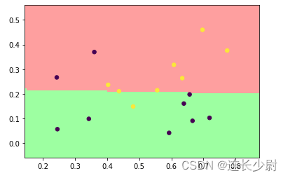
首先，用线性核进行训练，得到如下结果：

Accuracy = 82.3529% (14/17) (classification)

然后，将线性核改为高斯核，再次运行：

Accuracy = 82.3529% (14/17) (classification)

这里可以通过提高参数C来提高高斯核分类的准确率。
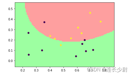
将C修改为10000：

model = svm_train(train_label, train_value, '-t 2 -c 10000')

再次运行：

Accuracy = 100% (17/17) (classification)

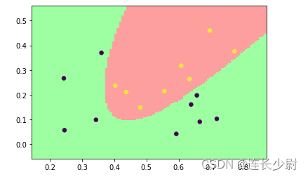
通过观察可以发现，由于训练集在二维特征空间中线性不可分，所以使用线性核无法全部分类正确，而使用高斯核可以将二维特征点升高维度，从而让这些点在高维空间中线性可分。同时，随着参数C的提高，分类错误代价会提高，训练过程中，超平面会尽可能的将训练集全部分开，但会有过拟合的风险。