1 参考论文

Fault diagnosis for small samples based on attention mechanism

2 开源代码

https://github.com/liguge/Fault-diagnosis-for-small-samples-based-on-attention-mechanism

3.摘要

针对深度学习在故障诊断中的应用，机械旋转设备部件在复杂的工作环境下容易发生故障，工业大数据存在标记样本有限、工作条件不同、噪声等问题。针对上述问题，提出了一种基于双路径卷积与注意机制(DCA)和双向门控循环单元(DCA- bigru)的小样本故障诊断方法，该方法的性能可以通过最新的正则化训练策略进行有效挖掘。利用BiGRU实现时空特征融合，利用DCA提取融合了注意权的振动信号特征。此外，还将全局平均池化(GAP)应用于降维和故障诊断。实验表明，DCA-BiGRU具有出色的泛化能力和鲁棒性，能够有效地进行各种复杂情况下的诊断。

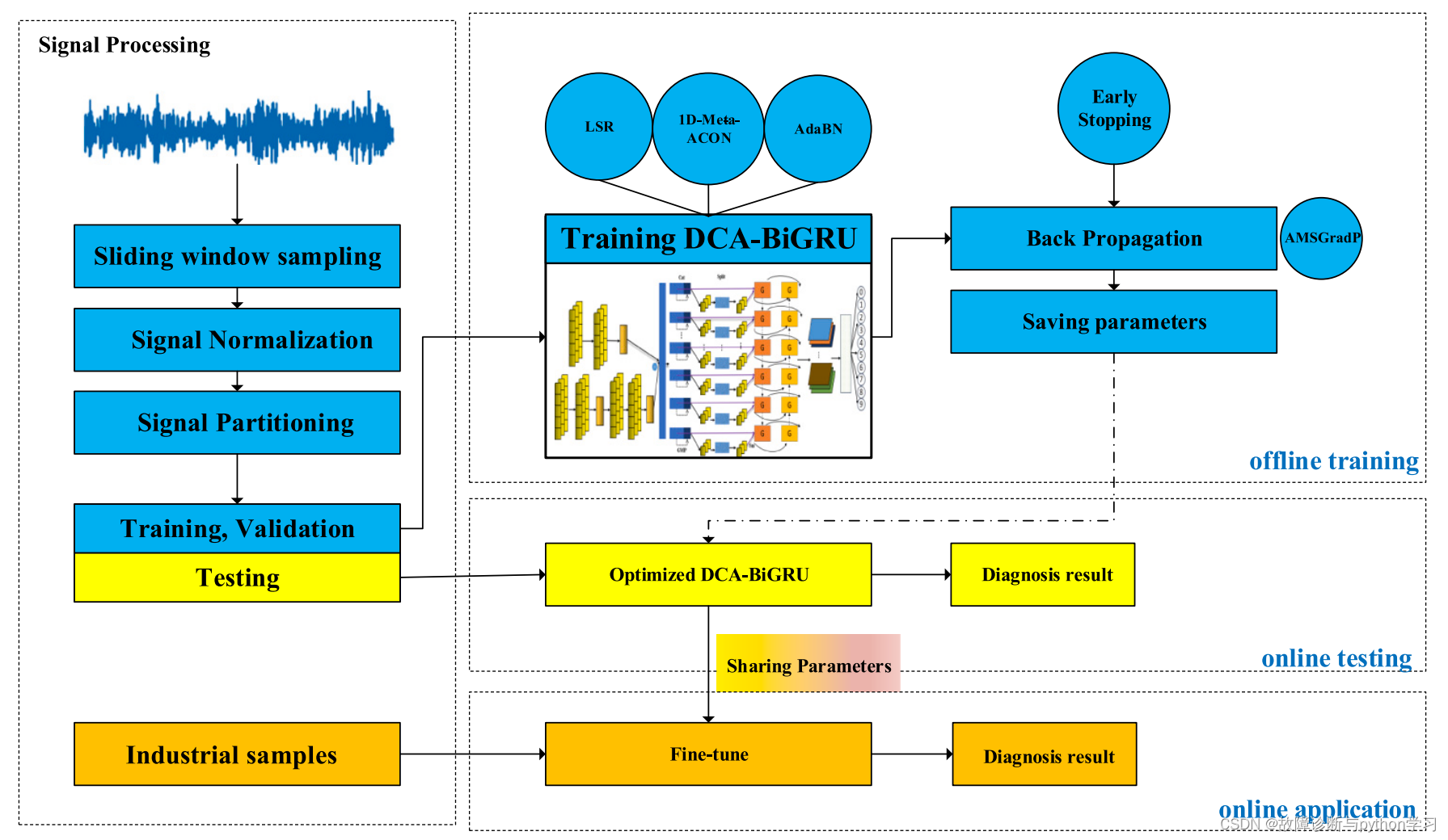
4.故障诊断流程图

5.网络模型

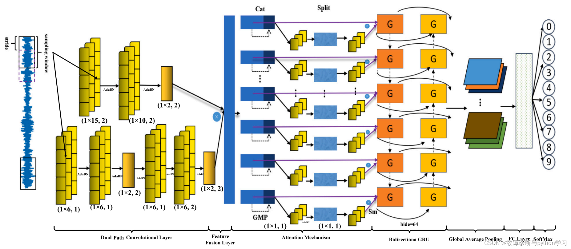
6.网络结构简介

输入1维数据：[batch_size, 1, 1024]–>双通道卷积–>特征融合（cat）–>注意力机制–>Bidirection GRU–>全局平均池化（Global average pool）–>全连接层–>softmax求分类概率

7.网络模型代码

建议使用pytorch，jupyter notebook

7.1MetaAconC

模块代码

import torch
from torch import nn
class AconC(nn.Module):
    r""" ACON activation (activate or not).
    # AconC: (p1*x-p2*x) * sigmoid(beta*(p1*x-p2*x)) + p2*x, beta is a learnable parameter
    # according to "Activate or Not: Learning Customized Activation" <https://arxiv.org/pdf/2009.04759.pdf>.
    """

    def __init__(self, width):
        super().__init__()
        self.p1 = nn.Parameter(torch.randn(1, width, 1))
        self.p2 = nn.Parameter(torch.randn(1, width, 1))
        self.beta = nn.Parameter(torch.ones(1, width, 1))
    def forward(self, x):
        return (self.p1 * x - self.p2 * x) * torch.sigmoid(self.beta * (self.p1 * x - self.p2 * x)) + self.p2 * x


class MetaAconC(nn.Module):
    r""" ACON activation (activate or not).
    # MetaAconC: (p1*x-p2*x) * sigmoid(beta*(p1*x-p2*x)) + p2*x, beta is generated by a small network
    # according to "Activate or Not: Learning Customized Activation" <https://arxiv.org/pdf/2009.04759.pdf>.
    """

    def __init__(self, width, r=16):
        super().__init__()
        self.fc1 = nn.Conv1d(width, max(r, width // r), kernel_size=1, stride=1, bias=True)
        self.bn1 = nn.BatchNorm1d(max(r, width // r), track_running_stats=True)
        self.fc2 = nn.Conv1d(max(r, width // r), width, kernel_size=1, stride=1, bias=True)
        self.bn2 = nn.BatchNorm1d(width, track_running_stats=True)
        self.p1 = nn.Parameter(torch.randn(1, width, 1))
        self.p2 = nn.Parameter(torch.randn(1, width, 1))

    def forward(self, x):
        beta = torch.sigmoid(self.bn2(self.fc2(self.bn1(self.fc1(x.mean(dim=2, keepdims=True))))))
        return (self.p1 * x - self.p2 * x) * torch.sigmoid(beta * (self.p1 * x - self.p2 * x)) + self.p2 * x

代码测试

x = torch.randn(16, 64, 1024)  #假设输入x：batch_size=16, channel=64, length=1024
Meta = MetaAconC(64)  #创建对象时需输入参数width，其为输入数据的channel
y = Meta(x)
print(y.shape)

>>>output
x.shape: torch.Size([16, 64, 1024])
y.shape: torch.Size([16, 64, 1024])

由结果可见，输入x的shape与输出y的shape是相同的

7.2注意力机制

注意力机制结构图

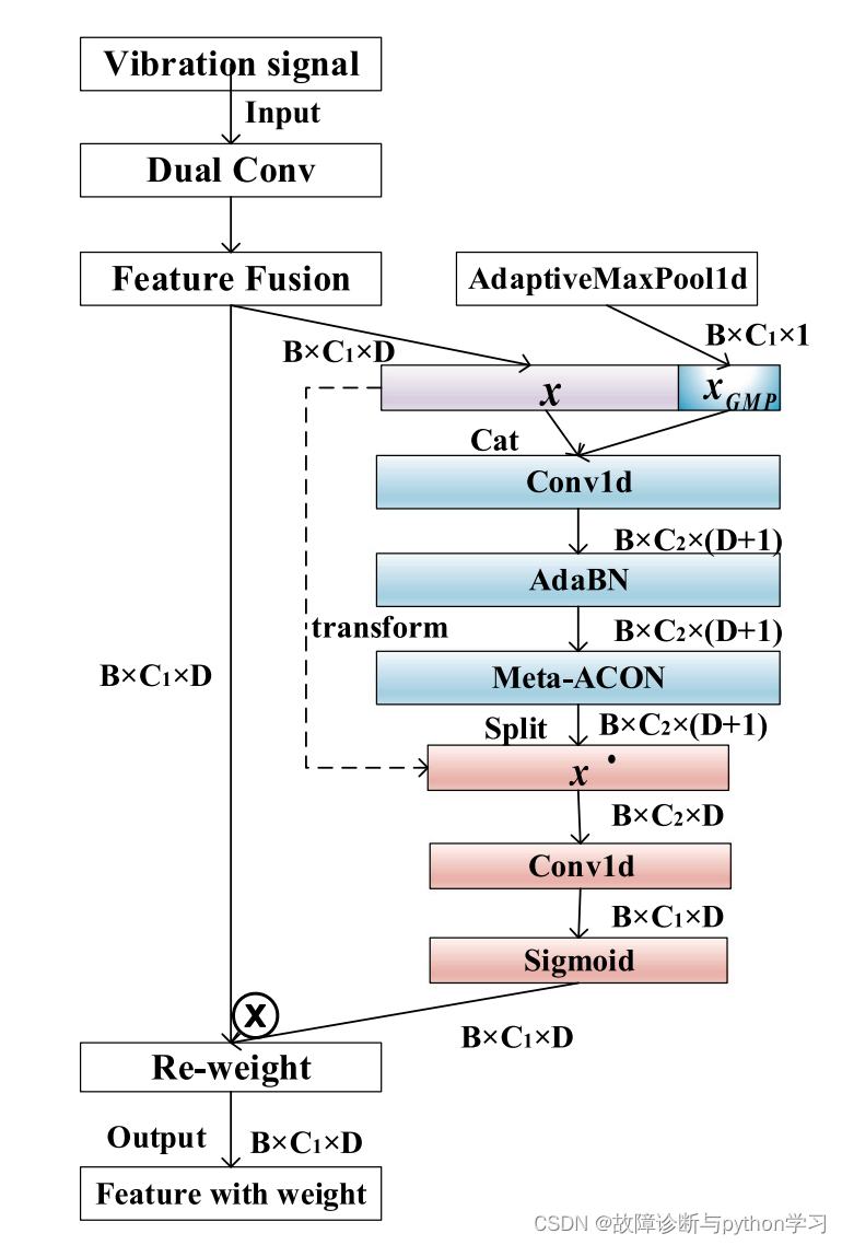
模块代码

class CoordAtt(nn.Module):
    def __init__(self, inp, oup, reduction=32):
        super(CoordAtt, self).__init__()
        # self.pool_w = nn.AdaptiveAvgPool1d(1)
        self.pool_w = nn.AdaptiveMaxPool1d(1)
        mip = max(6, inp // reduction)
        self.conv1 = nn.Conv1d(inp, mip, kernel_size=1, stride=1, padding=0)
        self.bn1 = nn.BatchNorm1d(mip, track_running_stats=False)
        self.act = MetaAconC(mip)
        self.conv_w = nn.Conv1d(mip, oup, kernel_size=1, stride=1, padding=0)

    def forward(self, x):
        identity = x
        n, c, w = x.size()
        x_w = self.pool_w(x)
        y = torch.cat([identity, x_w], dim=2)
        y = self.conv1(y)
        y = self.bn1(y)
        y = self.act(y)
        x_ww, x_c = torch.split(y, [w, 1], dim=2)
        a_w = self.conv_w(x_ww)
        a_w = a_w.sigmoid()
        out = identity * a_w
        return out

模块代码测试

x = torch.randn(16, 64, 1024)  #假设输入x：batch_size=16, channel=64, length=1024
Att = CoordAtt(inp=64, oup=64)  #创建注意力机制对象，输入参数inp和oup参数分别为channel
y = Att(x)
print('y.shape:',y.shape)

>>>output
y.shape: torch.Size([16, 64, 1024])

由结果可见，输入x的shape与输出y的shape是相同的

7.3 BiGRU测试

BiGRU结构图

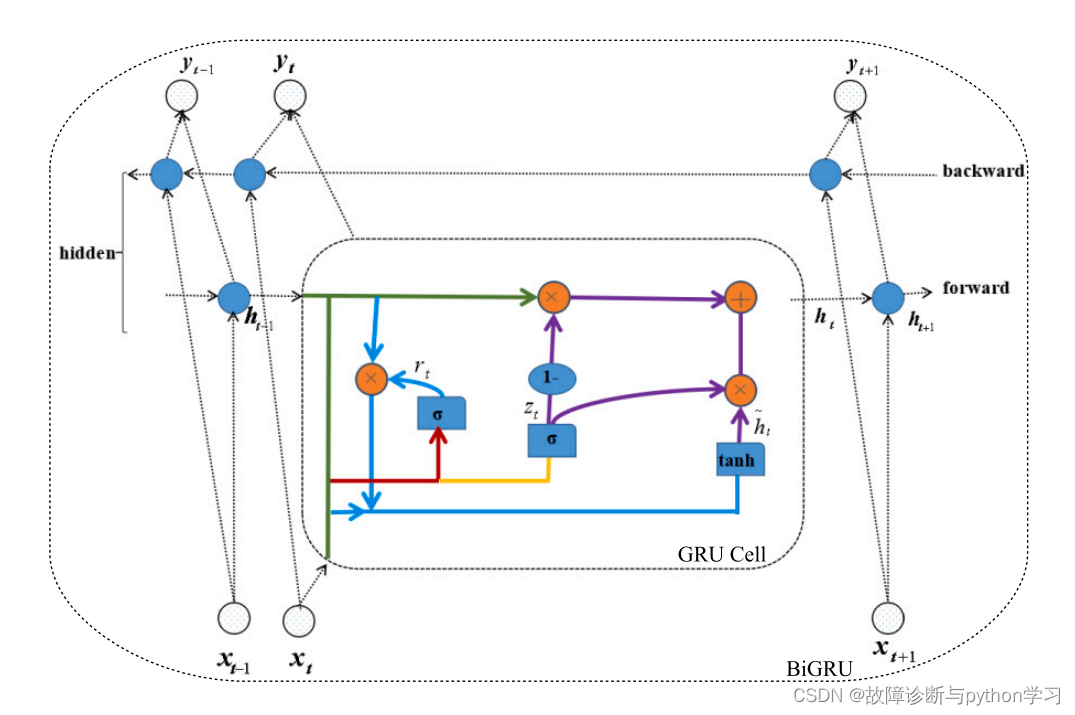
x = torch.randn(16, 64, 128)  #假设输入x：batch_size=16, channel=64, length=128
gru = nn.GRU(128, 64, bidirectional=True)  #创建GRU对象，128是输入数据x的长度；
                                           #如果bidirectional为False，64是输出数据的长度；如果bidirectional为True，则输出长度为64*2
y = gru(x)
print('y的值：\n',y)
print('y[0]的shape',y[0].shape)

>>>output
y的值：
 (tensor([[[-0.7509, -0.0468,  0.2881,  ..., -0.6559,  0.5780,  0.3481],
         [ 0.4099,  0.1912, -0.2534,  ..., -0.2067, -0.1099, -0.3594],
         [ 0.0275,  0.0937, -0.4309,  ..., -0.6266,  0.5375,  0.2510],
         ...,
         [-0.1896, -0.0118, -0.4895,  ...,  0.2022,  0.3144,  0.1806],
         [-0.5026,  0.4926, -0.2578,  ..., -0.3386, -0.3908, -0.1203],
         [-0.0431, -0.1084,  0.4494,  ...,  0.4320, -0.2916,  0.4126]]],
       grad_fn=<StackBackward0>))
y[0]的shape torch.Size([16, 64, 128])

由结果可以看出，y的输出为一个tuple元组类型，因此使用了y[0]获取里面的tensor数据。

7.4 全局平均池化GAP测试

# 第一步输入x 
x = torch.randn(16, 64, 32) #假设输入x：batch_size=16, channel=64, length=128
print('x的值:\n',x)
print('x[0][0]的值:',x[0][0])
print('x[0][0]的平均值:',torch.mean(x[0][0]))

# 第二步进行自适应平均池化
adavp = nn.AdaptiveAvgPool1d(1) #
y = adavp(x)
print('y的值:',y)
print('y的shape:',y.shape)

# 第三步
z = y.squeeze()
print('z的shape:',z.shape)

x的值:
 tensor([[[ 7.8979e-01,  1.3657e-01, -9.9066e-01,  ...,  9.5261e-01,
           9.8295e-02,  6.5511e-01],
         [-3.5707e-01, -2.3277e+00, -3.2558e-01,  ..., -2.2010e-01,
          -1.6210e+00, -1.2564e+00],
         [ 1.0400e+00, -1.8403e-01,  1.1634e+00,  ...,  5.7404e-02,
          -7.0334e-01, -1.5286e-01],
         ...,
         [-1.7541e+00,  5.9410e-01, -1.3539e-01,  ...,  8.6600e-02,
           1.2851e+00, -2.1541e+00],
         [ 1.6649e+00, -3.0008e+00, -6.5557e-01,  ...,  3.8984e-01,
          -2.4122e+00,  1.3892e+00],
         [ 3.2660e-01,  1.4245e+00,  8.2627e-01,  ..., -1.1504e+00,
           8.5084e-01, -2.3794e-02]]])
x[0][0]的值: tensor([ 0.7898,  0.1366, -0.9907, -0.9970,  1.6666, -1.5021,  0.9952,  0.5044,
         0.0828,  1.1746, -1.1589, -1.2519, -1.6039, -0.9943,  0.4700, -0.5370,
         0.5983, -0.6333, -1.3765, -0.9212, -0.3939, -0.7217,  0.4318,  0.4706,
         0.6322, -0.4217, -1.0003,  1.6015,  0.5162,  0.9526,  0.0983,  0.6551])
x[0][0]的平均值: tensor(-0.0852)
y的值: tensor([[[-0.0852],
         [-0.6024],
         [-0.0316],
         ...,
         [ 0.0157],
         [-0.2135],
         [ 0.1926]]])
y的shape: torch.Size([16, 64, 1])
z的shape: torch.Size([16, 64])

由结果可以看出，输入数据x1.shape=[16, 64, 32]全局平均池化是将输入数据的最后一维，及32个数据点取平均值。得到[16, 64]

7.5 整体网络测试

整体网络代码

class Net(nn.Module):
    def __init__(self):
        super(Net, self).__init__()
        self.p1_1 = nn.Sequential(nn.Conv1d(in_channels=1, out_channels=50, kernel_size=18, stride=2),
                                  nn.BatchNorm1d(50, track_running_stats=False),
                                  MetaAconC(50))
        self.p1_2 = nn.Sequential(nn.Conv1d(50, 30, kernel_size=10, stride=2),
                                  nn.BatchNorm1d(30, track_running_stats=False),
                                  MetaAconC(30))
        self.p1_3 = nn.MaxPool1d(2, 2)
        self.p2_1 = nn.Sequential(nn.Conv1d(1, 50, kernel_size=6, stride=1),
                                  nn.BatchNorm1d(50, track_running_stats=False),
                                  MetaAconC(50))
        self.p2_2 = nn.Sequential(nn.Conv1d(50, 40, kernel_size=6, stride=1),
                                  nn.BatchNorm1d(40, track_running_stats=False),
                                  MetaAconC(40))
        self.p2_3 = nn.MaxPool1d(2, 2)
        self.p2_4 = nn.Sequential(nn.Conv1d(40, 30, kernel_size=6, stride=1), nn.BatchNorm1d(30, track_running_stats=False),MetaAconC(30))
        self.p3_0 = CoordAtt(30, 30)
        self.p2_5 = nn.Sequential(nn.Conv1d(30, 30, kernel_size=6, stride=2),
                                  nn.BatchNorm1d(30, track_running_stats=False),
                                  MetaAconC(30))
        self.p2_6 = nn.MaxPool1d(2, 2)
        
        self.p3_1 = nn.Sequential(nn.GRU(124, 64, bidirectional=True))  #
        # self.p3_2 = nn.Sequential(nn.LSTM(128, 512))
        self.p3_3 = nn.Sequential(nn.AdaptiveAvgPool1d(1))  #GAP
        self.p4 = nn.Sequential(nn.Linear(30, 10))

    def forward(self, x):
        p1 = self.p1_3(self.p1_2(self.p1_1(x)))
        print('p1.shape:',p1.shape)
        
        p2 = self.p2_6(self.p2_5(self.p2_4(self.p2_3(self.p2_2(self.p2_1(x))))))
        print('p2.shape:',p2.shape)
        
        encode = torch.mul(p1, p2)
        print('encode.shape:',encode.shape)
        
        # p3 = self.p3_2(self.p3_1(encode))
        p3_0 = self.p3_0(encode).permute(1, 0, 2)
        print('p3_0.shape:',p3_0.shape)
        
        p3_2, _ = self.p3_1(p3_0)
        print('p3_2.shape:',p3_2.shape)
        
        # p3_2, _ = self.p3_2(p3_1)
        p3_11 = p3_2.permute(1, 0, 2)  # 
        print('p3_11.shape:',p3_11.shape)
        
        p3_12 = self.p3_3(p3_11).squeeze()
        print('p3_12.shape:',p3_12.shape)
        # p3_11 = h1.permute(1,0,2)
        # p3 = self.p3(encode)
        # p3 = p3.squeeze()
        # p4 = self.p4(p3_11)  # LSTM(seq_len, batch, input_size)
        # p4 = self.p4(encode)
        p4 = self.p4(p3_12)
        print('p4.shape:',p4.shape)
        return p4

代码测试

model = Net() 
x = torch.randn(16, 1, 1024) #假设输入x：batch_size=16, channel=1, length=1024
y = model(x)

>>>output
p1.shape: torch.Size([16, 30, 124])
p2.shape: torch.Size([16, 30, 124])
encode.shape: torch.Size([16, 30, 124])
p3_0.shape: torch.Size([30, 16, 124])
p3_2.shape: torch.Size([30, 16, 128])
p3_11.shape: torch.Size([16, 30, 128])
p3_12.shape: torch.Size([16, 30])
p4.shape: torch.Size([16, 10])

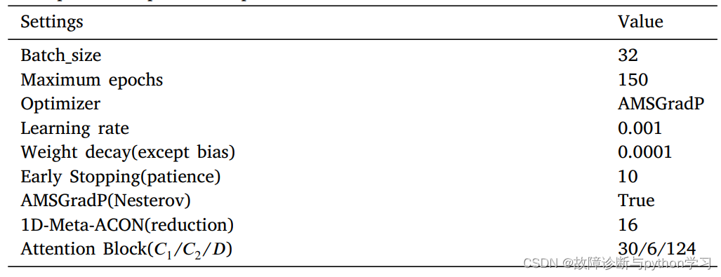
8 实验设置

8.1 模型参数设置

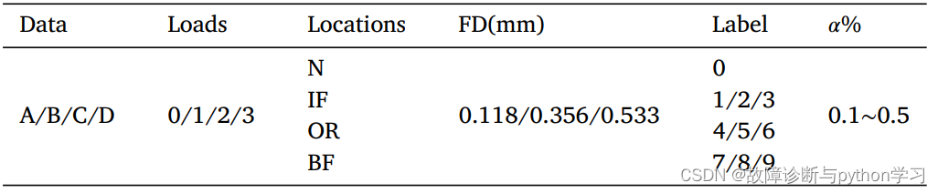
8.2 实验数据设置

9 实验验证

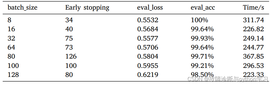
案例1：CWRU

不同batch_size下的结果

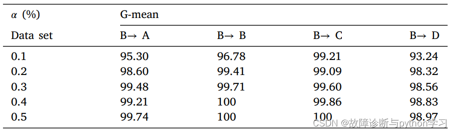
不同负载下的结果

（后续继续完善）

注：
① 若本论文对你有帮助启发，建议引用本论文~
② 欢迎关注公众号《故障诊断与Python学习》
③ 若有好的开源代码，欢迎后台联系推荐~