UMAP降维算法原理详解和应用示例
降维不仅仅是为了数据可视化。它还可以识别高维空间中的关键结构并将它们保存在低维嵌入中来克服“维度诅咒”本文将介绍一种流行的降维技术Uniform Manifold Approximation and Projection(UMAP)的内部工作原理,并提供一个 Python 示例。(UMAP) 如何工作的?分析 UMAP 名称让我们从剖析 UMAP 名称开始,这将使我们对算法应该做什么有一个大致的了
降维不仅仅是为了数据可视化。它还可以识别高维空间中的关键结构并将它们保存在低维嵌入中来克服“维度诅咒”
本文将介绍一种流行的降维技术Uniform Manifold Approximation and Projection (UMAP)的内部工作原理,并提供一个 Python 示例。
(UMAP) 如何工作的?
分析 UMAP 名称
让我们从剖析 UMAP 名称开始,这将使我们对算法应该做什么有一个大致的了解。
以下描述不是官方定义,而是我总结出来的可帮助我们理解 UMAP 的要点。
Projection ——通过投影点在平面、曲面或线上再现空间对象的过程或技术。也可以将其视为对象从高维空间到低维空间的映射。
Approximation——算法假设我们只有一组有限的数据样本(点),而不是构成流形的整个集合。因此,我们需要根据可用数据来近似流形。
Manifold——流形是一个拓扑空间,在每个点附近局部类似于欧几里得空间。一维流形包括线和圆,但不包括类似数字8的形状。二维流形(又名曲面)包括平面、球体、环面等。
Uniform——均匀性假设告诉我们我们的数据样本均匀(均匀)分布在流形上。但是,在现实世界中,这种情况很少发生。因此这个假设引出了在流形上距离是变化的概念。即,空间本身是扭曲的:空间根据数据显得更稀疏或更密集的位置进行拉伸或收缩。
综上所述,我们可以将UMAP描述为:
一种降维技术,假设可用数据样本均匀(Uniform)分布在拓扑空间(Manifold)中,可以从这些有限数据样本中近似(Approximation)并映射(Projection)到低维空间。
上面对算法的描述可能会对我们理解它的原理有一点帮助,但是对于UMAP是如何实现的仍然没有说清楚。为了回答“如何”的问题,让我们分析UMAP执行的各个步骤。
UMAP执行的步骤
我们可以将UMAP分为两个主要步骤:
- 学习高维空间中的流形结构
- 找到该流形的低维表示。
下面我们将把它分解成更小的部分,以加深我们对算法的理解。下面的地图显示了我们在分析每个部分工作流程。

1 — 学习流形结构
在我们将数据映射到低维之前,肯定首先需要弄清楚它在高维空间中的样子。
1.1.寻找最近的邻居
UMAP 首先使用 Nearest-Neighbor-Descent 算法找到最近的邻居。我们可以通过调整 UMAP 的 n_neighbors 超参数来指定我们想要使用多少个近邻点。
试验 n_neighbors 的数量很重要,因为它控制 UMAP 如何平衡数据中的局部和全局结构。它通过在尝试学习流形结构时限制局部邻域的大小来实现。
本质上,一个小的n_neighbors 值意味着我们需要一个非常局部的解释,准确地捕捉结构的细节。而较大的 n_neighbors 值意味着我们的估计将基于更大的区域,因此在整个流形中更广泛地准确。
1.2.构建一个图
接下来,UMAP 需要通过连接之前确定的最近邻来构建图。为了理解这个过程,我们需要将他分成几个子步骤来解释邻域图是如何形成的。
1.2.1 变化距离
正如对 UMAP 名称的分析所述,我们假设点在流形上均匀分布,这表明它们之间的空间根据数据看起来更稀疏或更密集的位置而拉伸或收缩的。
它本质上意味着距离度量不是在整个空间中通用的,而是在不同区域之间变化的。我们可以通过在每个数据点周围绘制圆圈/球体来对其进行可视化,由于距离度量的不同,它们的大小似乎不同(见下图)。

1.2.2 local_connectivity
接下来,我们要确保试图学习的流形结构不会导致许多不连通点。所以需要使用另一个超参数local_connectivity(默认值= 1)来解决这个潜在的问题
当我们设置local_connectivity=1 时,我们告诉高维空间中的每一个点都与另一个点相关联。
1.2.3 模糊区域
你一定已经注意到上面的图也包含了模糊的圆圈延伸到最近的邻居之外。这告诉我们,当我们离感兴趣的点越远,与其他点联系的确定性就越小。
这两个超参数(local_connectivity 和 n_neighbors)最简单的理解就是可以将他们视为下限和上限:
Local_connectivity(默认值为1):100%确定每个点至少连接到另一个点(连接数量的下限)。
n_neighbors(默认值为15):一个点直接连接到第 16 个以上的邻居的可能性为 0%,因为它在构建图时落在 UMAP 使用的局部区域之外。
2 到 15 : 有一定程度的确定性(>0% 但 <100%)一个点连接到它的第 2 个到第 15 个邻居。

1.2.4 边的合并
最后,我们需要了解上面讨论的连接确定性是通过边权重(w)来表达的。
由于我们采用了不同距离的方法,因此从每个点的角度来看,我们不可避免地会遇到边缘权重不对齐的情况。 例如,点 A→B 的边权重与 B→A 的边权重不同。

UMAP 通过取两条边的并集克服了我们刚刚描述的边权重不一致的问题。 UMAP 文档解释如下:
如果我们想将权重为 a 和 b 的两条不同的边合并在一起,那么我们应该有一个权重为 𝑎+𝑏−𝑎⋅𝑏 的单边。 考虑这一点的方法是,权重实际上是边(1-simplex)存在的概率。 组合权重就是至少存在一条边的概率。
最后,我们得到一个连接的邻域图,如下所示:

2 — 寻找低维表示
从高维空间学习近似流形后,UMAP 的下一步是将其投影(映射)到低维空间。
2.1.最小距离
与第一步不同,我们不希望在低维空间表示中改变距离。相反,我们希望流形上的距离是相对于全局坐标系的标准欧几里得距离。
从可变距离到标准距离的转换的转换也会影响与最近邻居的距离。因此,我们必须传递另一个名为 min_dist(默认值=0.1)的超参数来定义嵌入点之间的最小距离。
本质上,我们可以控制点的最小分布,避免在低维嵌入中许多点相互重叠的情况。
2.2.最小化成本函数(Cross-Entropy)
指定最小距离后,该算法可以开始寻找较好的低维流形表示。 UMAP 通过最小化以下成本函数(也称为交叉熵 (CE))来实现:

最终目标是在低维表示中找到边的最优权值。这些最优权值随着上述交叉熵函数的最小化而出现,这个过程是可以通过随机梯度下降法来进行优化的
就是这样!UMAP的工作现在完成了,我们得到了一个数组,其中包含了指定的低维空间中每个数据点的坐标。
Python中使用UMAP
上面我们已经介绍UMAP的知识点,现在我们在Python中进行实践。
我们将在MNIST数据集(手写数字的集合)上应用UMAP,以说明我们如何成功地分离数字并在低维空间中显示它们。
我们将使用以下数据和库:
1、Scikit-learn库,MNIST数字数据(load_digits);将数据分割为训练和测试样本(train_test_split);
2、UMAP库执行降维;
3、Plotly和Matplotlib用于数据可视化;
4、Pandas和Numpy用于数据操作。
第一步是导入上面列出的库。
# Data manipulation
import pandas as pd # for data manipulation
import numpy as np # for data manipulation

# Visualization
import plotly.express as px # for data visualization
import matplotlib.pyplot as plt # for showing handwritten digits

# Skleran
from sklearn.datasets import load_digits # for MNIST data
from sklearn.model_selection import train_test_split # for splitting data into train and test samples

# UMAP dimensionality reduction
from umap import UMAP
接下来,我们加载MNIST数据并显示前10个手写数字的图像。
# Load digits data
digits = load_digits()

# Load arrays containing digit data (64 pixels per image) and their true labels
X, y = load_digits(return_X_y=True)

# Some stats
print('Shape of digit images: ', digits.images.shape)
print('Shape of X (main data): ', X.shape)
print('Shape of y (true labels): ', y.shape)

# Display images of the first 10 digits
fig, axs = plt.subplots(2, 5, sharey=False, tight_layout=True, figsize=(12,6), facecolor='white')
n=0
plt.gray()
for i in range(0,2):
    for j in range(0,5):
        axs[i,j].matshow(digits.images[n])
        axs[i,j].set(title=y[n])
        n=n+1
plt.show()

接下来,我们将创建一个用于绘制3D散点图的函数,我们可以多次重用该函数来显示UMAP降维的结果。
def chart(X, y):
    #--------------------------------------------------------------------------#
    # This section is not mandatory as its purpose is to sort the data by label
    # so, we can maintain consistent colors for digits across multiple graphs

    # Concatenate X and y arrays
    arr_concat=np.concatenate((X, y.reshape(y.shape[0],1)), axis=1)
    # Create a Pandas dataframe using the above array
    df=pd.DataFrame(arr_concat, columns=['x', 'y', 'z', 'label'])
    # Convert label data type from float to integer
    df['label'] = df['label'].astype(int)
    # Finally, sort the dataframe by label
    df.sort_values(by='label', axis=0, ascending=True, inplace=True)
    #--------------------------------------------------------------------------#

    # Create a 3D graph
    fig = px.scatter_3d(df, x='x', y='y', z='z', color=df['label'].astype(str), height=900, width=950)

    # Update chart looks
    fig.update_layout(title_text='UMAP',
                      showlegend=True,
                      legend=dict(orientation="h", yanchor="top", y=0, xanchor="center", x=0.5),
                      scene_camera=dict(up=dict(x=0, y=0, z=1),
                                            center=dict(x=0, y=0, z=-0.1),
                                            eye=dict(x=1.5, y=-1.4, z=0.5)),
                                            margin=dict(l=0, r=0, b=0, t=0),
                      scene = dict(xaxis=dict(backgroundcolor='white',
                                              color='black',
                                              gridcolor='#f0f0f0',
                                              title_font=dict(size=10),
                                              tickfont=dict(size=10),
                                             ),
                                   yaxis=dict(backgroundcolor='white',
                                              color='black',
                                              gridcolor='#f0f0f0',
                                              title_font=dict(size=10),
                                              tickfont=dict(size=10),
                                              ),
                                   zaxis=dict(backgroundcolor='lightgrey',
                                              color='black',
                                              gridcolor='#f0f0f0',
                                              title_font=dict(size=10),
                                              tickfont=dict(size=10),
                                             )))
    # Update marker size
    fig.update_traces(marker=dict(size=3, line=dict(color='black', width=0.1)))

    fig.show()
将 UMAP 应用于我们的数据
现在,我们将之前加载到 X 中的 MNIST 数字数据。 X (1797,64) 的形状告诉我们我们有 1,797 个数字,每个数字由 64 个维度组成。
我们将使用 UMAP 将维数从 64 降到 3。我已经列出了 UMAP 中可用的每个超参数,并简要说明了它们的作用。
虽然在本示例中,我将大部分超参数设置为默认值,但你可以尝试改变它们来查看它们如何影响结果。
# Configure UMAP hyperparameters
reducer = UMAP(n_neighbors=100, # default 15, The size of local neighborhood (in terms of number of neighboring sample points) used for manifold approximation.
               n_components=3, # default 2, The dimension of the space to embed into.
               metric='euclidean', # default 'euclidean', The metric to use to compute distances in high dimensional space.
               n_epochs=1000, # default None, The number of training epochs to be used in optimizing the low dimensional embedding. Larger values result in more accurate embeddings.
               learning_rate=1.0, # default 1.0, The initial learning rate for the embedding optimization.
               init='spectral', # default 'spectral', How to initialize the low dimensional embedding. Options are: {'spectral', 'random', A numpy array of initial embedding positions}.
               min_dist=0.1, # default 0.1, The effective minimum distance between embedded points.
               spread=1.0, # default 1.0, The effective scale of embedded points. In combination with ``min_dist`` this determines how clustered/clumped the embedded points are.
               low_memory=False, # default False, For some datasets the nearest neighbor computation can consume a lot of memory. If you find that UMAP is failing due to memory constraints consider setting this option to True.
               set_op_mix_ratio=1.0, # default 1.0, The value of this parameter should be between 0.0 and 1.0; a value of 1.0 will use a pure fuzzy union, while 0.0 will use a pure fuzzy intersection.
               local_connectivity=1, # default 1, The local connectivity required -- i.e. the number of nearest neighbors that should be assumed to be connected at a local level.
               repulsion_strength=1.0, # default 1.0, Weighting applied to negative samples in low dimensional embedding optimization.
               negative_sample_rate=5, # default 5, Increasing this value will result in greater repulsive force being applied, greater optimization cost, but slightly more accuracy.
               transform_queue_size=4.0, # default 4.0, Larger values will result in slower performance but more accurate nearest neighbor evaluation.
               a=None, # default None, More specific parameters controlling the embedding. If None these values are set automatically as determined by ``min_dist`` and ``spread``.
               b=None, # default None, More specific parameters controlling the embedding. If None these values are set automatically as determined by ``min_dist`` and ``spread``.
               random_state=42, # default: None, If int, random_state is the seed used by the random number generator;
               metric_kwds=None, # default None) Arguments to pass on to the metric, such as the ``p`` value for Minkowski distance.
               angular_rp_forest=False, # default False, Whether to use an angular random projection forest to initialise the approximate nearest neighbor search.
               target_n_neighbors=-1, # default -1, The number of nearest neighbors to use to construct the target simplcial set. If set to -1 use the ``n_neighbors`` value.
               #target_metric='categorical', # default 'categorical', The metric used to measure distance for a target array is using supervised dimension reduction. By default this is 'categorical' which will measure distance in terms of whether categories match or are different.
               #target_metric_kwds=None, # dict, default None, Keyword argument to pass to the target metric when performing supervised dimension reduction. If None then no arguments are passed on.
               #target_weight=0.5, # default 0.5, weighting factor between data topology and target topology.
               transform_seed=42, # default 42, Random seed used for the stochastic aspects of the transform operation.
               verbose=False, # default False, Controls verbosity of logging.
               unique=False, # default False, Controls if the rows of your data should be uniqued before being embedded.
              )

# Fit and transform the data
X_trans = reducer.fit_transform(X)

# Check the shape of the new data
print('Shape of X_trans: ', X_trans.shape)
以上代码将UMAP应用于我们的MNIST数据,并打印转换后的数组的形状,以确认我们已经成功地将维数从64降至3。

现在,我们可以使用前面创建的图表绘图功能来可视化我们的三维数字数据。我们用一行简单的代码调用函数,传递我们想要可视化的数组。

可以在这里查看:https://chart-studio.plotly.com/create/?fid=SolClover:166#/
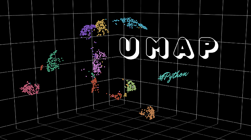
结果看起来非常好,数字集群之间有明显的分离。有趣的是,数字1形成了三个不同的集群,这可以用人们书写数字1的不同方式来解释:

注意,1的底数和数字2的底数很像。我们可以在一小簇红色的1中找到这些案例,它与绿色的2非常接近。
监督的UMAP
正如本文开头所提到的,我们还可以以监督的方式使用UMAP来帮助减少数据的维数。
在执行监督降维时,除了图像数据(X_train数组),我们还需要将标签数据(y_train数组)传递给fit_transform方法(参见下面的代码)。
另外,我对超参数做了一些其他的小修改,将min_dist=0.5和local_connectivity=2设置为更好的可视化和更好的测试示例结果。
# Split data into training and testing
X_train, X_test, y_train, y_test = train_test_split(X, y, test_size=0.25, shuffle=False)

# Configure UMAP hyperparameters
reducer2 = UMAP(n_neighbors=100, n_components=3, n_epochs=1000,
                min_dist=0.5, local_connectivity=2, random_state=42,
              )

# Training on MNIST digits data - this time we also pass the true labels to a fit_transform method
X_train_res = reducer2.fit_transform(X_train, y_train)

# Apply on a test set
X_test_res = reducer2.transform(X_test)

# Print the shape of new arrays
print('Shape of X_train_res: ', X_train_res.shape)
print('Shape of X_test_res: ', X_test_res.shape)

现在,我们已经成功地使用监督UMAP方法降维,我们可以绘制3D散点图来显示结果。
chart(X_train_res, y_train)

https://chart-studio.plotly.com/create/?fid=SolClover:169
我们可以看到,UMAP形成了非常紧密的簇,每个数字之间有相当大的距离。
现在,我们为测试数据创建相同的3D图,以查看UMAP是否能够成功地将新的数据点放置到这些集群中。
chart(X_test_res, y_test)

https://chart-studio.plotly.com/create/?fid=SolClover:172
结果非常好,只有几个数字放在了错误的簇中。特别的是,看起来算法在处理数字3时遇到了困难,有几个例子位于7、8和5的旁边。
总结
感谢您阅读这篇长文,我希望它的每一部分都能让您更深入地了解这个伟大的算法是如何运行的。
一般来说,UMAP具有坚实的数学基础,它通常比t-SNE等类似的降维算法做得更好。
UMAP的秘诀在于保持低维空间中相对全局距离的同时推断局部和全局结构的能力。这些能力使我们能够找到特定的解决方案,比如找到数字1和2的手写形式之间的相似之处。
作者:Saul Dobilas

为开发者提供学习成长、分享交流、生态实践、资源工具等服务,帮助开发者快速成长。
更多推荐


 33
33 2
2- 0


 已为社区贡献19条内容

所有评论(0)