六、二手房数据分析

六、二手房数据分析6.1 背景介绍6.1.1 实验背景随着房地产市场发展，房价越来越高。为了的到影响房价的增长因素，现在从数据角度出发，分析以下左右房价的因素。数据介绍CATE 城区bedrooms 卧室数量halls 客厅AREA 面积floor 地面高度，楼层subway 附近是否有地铁school 附近是否有学校price 价格名称DISTRICT区域6.2 载入数据6.2.1 导入支持库i

小石小石摩西摩西

35730人浏览 · 2021-08-16 09:27:52

小石小石摩西摩西 · 2021-08-16 09:27:52 发布

六、二手房数据分析

6.1 背景介绍

6.1.1 实验背景

随着房地产市场发展，房价越来越高。为了的到影响房价的增长因素，现在从数据角度出发，分析以下左右房价的因素。

数据介绍

CATE 城区
bedrooms 卧室数量
halls 客厅
AREA 面积
floor 地面高度，楼层
subway 附近是否有地铁
school 附近是否有学校
price 价格
名称
DISTRICT区域

6.2 载入数据

6.2.1 导入支持库

import math
import numpy as np
import pandas as pd
from pandas import Series,DataFrame
import matplotlib.pyplot as plt
import statsmodels.api as sm
from scipy import stats
from statsmodels.stats.outliers_influence import summary_table
from pylab import mpl
import copy

注：若没有statsmodels模块，请到Terminal用如下命令安装

sudo pip3 install statsmodels
# Terminal在jupyter首页NEW-Other-Terminal

6.2.2 载入数据

data_source='../data/housedata.csv'#数据源文件
df = pd.read_csv(data_source,encoding='UTF8') #读入二手房数据

6.2.3 设置中文显示

plt.rcParams['font.sans-serif']=['SimHei'] #用来正常显示中文标签
plt.rcParams['axes.unicode_minus']=False #用来正常显示负号

6.3 数据探查

6.3.1 查看数据源数据特征

df_ana = df
df_ana.head() # 样本取样

[外链图片转存失败,源站可能有防盗链机制,建议将图片保存下来直接上传(img-OaeDIcdE-1629077234143)(Matplotlib基础课程.assets/Matplotlib_09_1.png)]

6.3.2 继续检查样本数量

len(df_ana) # 样本数量

[外链图片转存失败,源站可能有防盗链机制,建议将图片保存下来直接上传(img-Vx99izwd-1629077234145)(Matplotlib基础课程.assets/Matplotlib_09_2.png)]

6.3.3 将价格单位转化为万元

df_ana['price'] = df_ana['price']/10000
df_ana.head()

[外链图片转存失败,源站可能有防盗链机制,建议将图片保存下来直接上传(img-UMvnRrbI-1629077234146)(Matplotlib基础课程.assets/Matplotlib_09_3.png)]

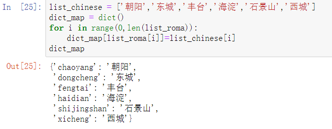
6.3.4 将CATE（城区）列转化为中文

list_roma = list(set(df_ana['CATE']))
list_roma.sort()
list_roma

[外链图片转存失败,源站可能有防盗链机制,建议将图片保存下来直接上传(img-UbpIYrsH-1629077234148)(Matplotlib基础课程.assets/Matplotlib_09_4.png)]

list_chinese = ['朝阳','东城','丰台','海淀','石景山','西城']
dict_map = dict()
for i in range(0,len(list_roma)):
    dict_map[list_roma[i]]=list_chinese[i]
dict_map

用汉字替换拼音：

for x in dict_map.keys():
    df_ana['CATE'] = df_ana['CATE'].str.replace(x,dict_map[x])
df_ana.head()

[外链图片转存失败,源站可能有防盗链机制,建议将图片保存下来直接上传(img-MttjmoX6-1629077234150)(Matplotlib基础课程.assets/Matplotlib_09_6.png)]

6.3.5 调整城区和楼层的因子水平顺序

df_ana = df_ana.sort_values(by = ['floor'],axis = 0,ascending = True)
df_ana.head()

[外链图片转存失败,源站可能有防盗链机制,建议将图片保存下来直接上传(img-neHNSOuM-1629077234150)(Matplotlib基础课程.assets/Matplotlib_09_7.png)]

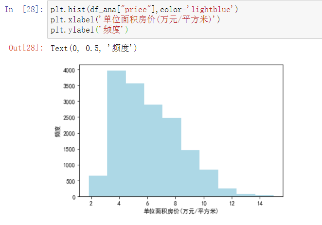
6.4 简单绘图分析

6.4.1 分析数据源，绘制因变量直方图

plt.hist(df_ana["price"],color='lightblue')
plt.xlabel('单位面积房价(万元/平方米)')
plt.ylabel('频度')

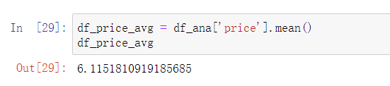
6.4.2 检查售价均值

df_price_avg = df_ana['price'].mean()
df_price_avg

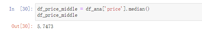
6.4.3 检查中位数

df_price_middle = df_ana['price'].median()
df_price_middle

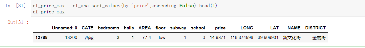
6.4.4 检查最大值

df_price_max = df_ana.sort_values(by='price',ascending=False).head(1)
df_price_max

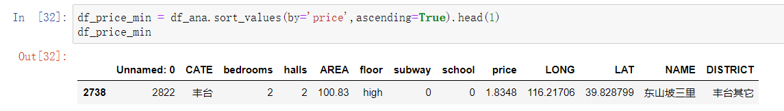
6.4.5 检查最小值

df_price_min = df_ana.sort_values(by='price',ascending=True).head(1)
df_price_min

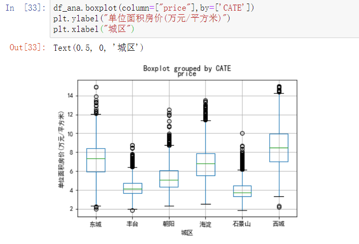
6.4.6 绘制房价的分组箱线图

df_ana.boxplot(column=["price"],by=['CATE'])
plt.ylabel("单位面积房价(万元/平方米)")
plt.xlabel("城区")

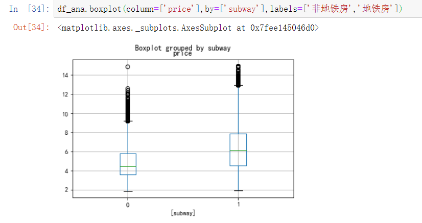
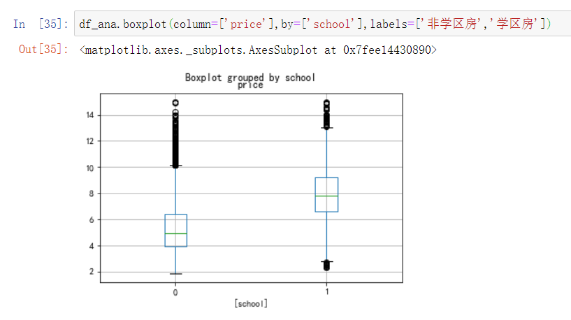
6.4.7 地铁、学区的分组箱线图

df_ana.boxplot(column=['price'],by=['subway'],labels=['非地铁房','地铁房'])

df_ana.boxplot(column=['price'],by=['school'],labels=['非学区房','学区房'])

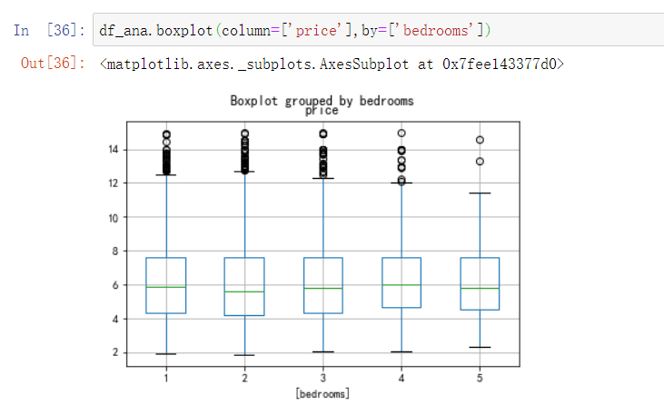
6.4.8 考察房源，客厅、卧室和楼层是否对价格有影响

df_ana.boxplot(column=['price'],by=['bedrooms'])

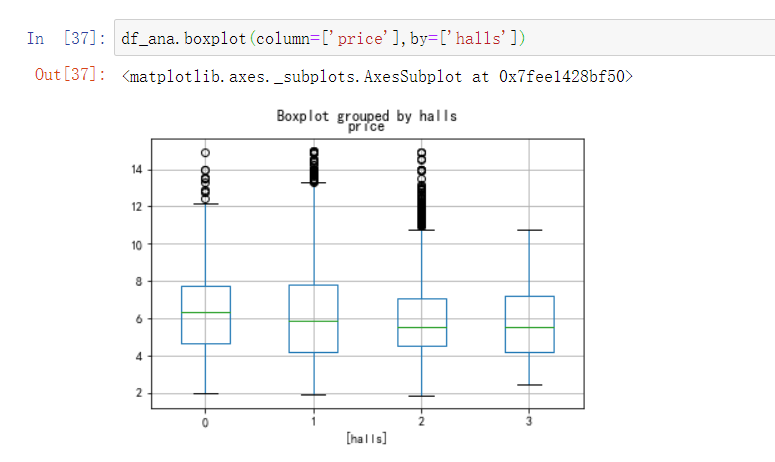
考察客厅数量对房价的影响：

df_ana.boxplot(column=['price'],by=['halls'])

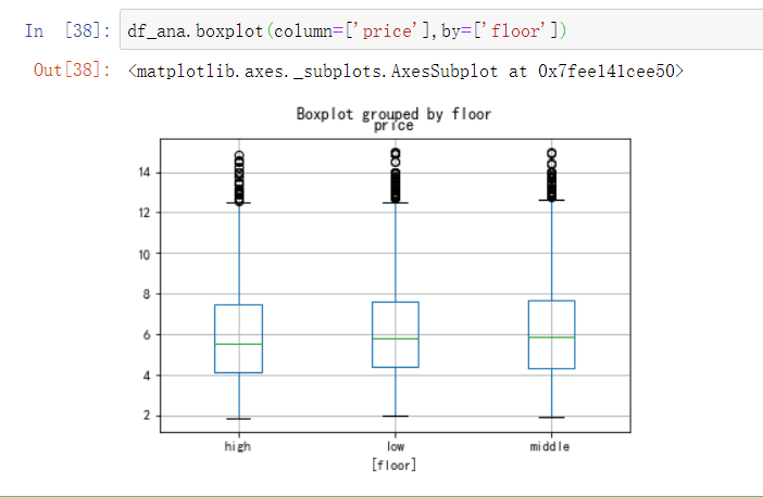
考察楼层高低对房价的影响：

df_ana.boxplot(column=['price'],by=['floor'])

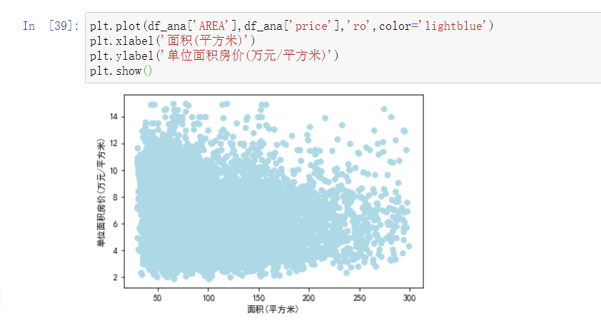
6.4.9 考察房屋面积和单位价格的关系

plt.plot(df_ana['AREA'],df_ana['price'],'ro',color='lightblue')
plt.xlabel('面积(平方米)')
plt.ylabel('单位面积房价(万元/平方米)')
plt.show()

6.4.10 建立线性回归模型

客厅数做因子化处理，变成二分变量，使得建模有更好的解读。

def fun(x):
    if isinstance(x,int): 
        if x == 0:
            return 0
        else:
            return 1
    else:
        return 0
style_halls = df_ana
df_ana['have_halls'] = df_ana['halls'].apply(lambda x: fun(x))
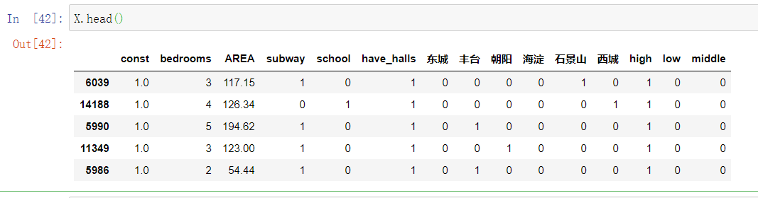
col_n =['CATE','bedrooms','AREA','floor','subway','school','have_halls']

将变量参数数据化

y=df_ana.price
x=pd.DataFrame(df_ana,columns=col_n)  #设置自变量x
x_dum_cate=pd.get_dummies(x['CATE'])  #对哑变量编码
x_dum_floor=pd.get_dummies(x['floor'])  #对哑变量编码
del x['CATE']
del x['floor']
x=pd.concat([x,x_dum_cate],axis=1)
x=pd.concat([x,x_dum_floor],axis=1)
X=sm.add_constant(x)  #增加截距项

查看数据：

X.head()

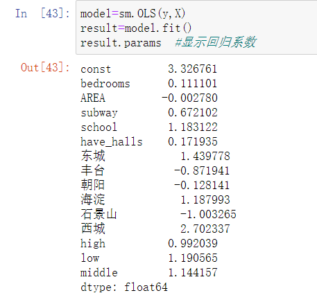
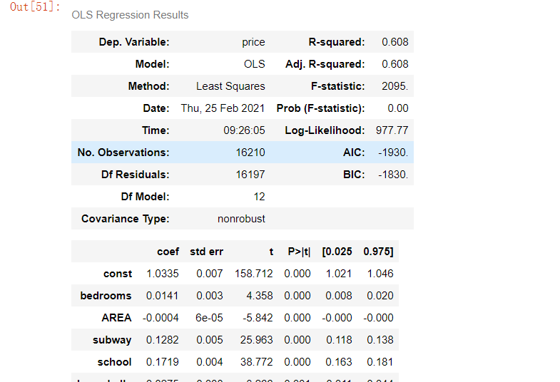
线性回归模型（因变量：单位面积房价）：

model=sm.OLS(y,X)
result=model.fit()
result.params  #显示回归系数

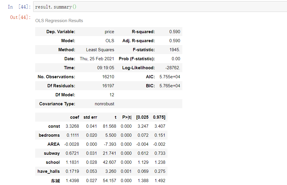
result.summary()

y_hat=result.predict(X)
residuals=y-y_hat
fig = plt.figure()

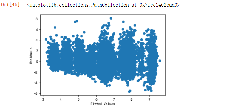
6.4.11 验证模型是否符合线性模型

fg1 = fig.add_subplot(221)
fg1.set_title('Residuals VS Fitted') 
plt.xlabel('Fitted Values')
plt.ylabel('Residuals')
plt.scatter(y_hat,residuals)

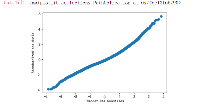
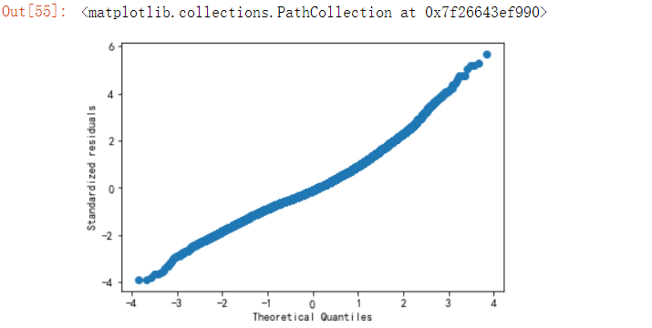
6.4.12 验证房价是否是正太分布

residuals_n=(residuals-np.mean(residuals))/np.std(residuals)
sorted_=np.sort(residuals_n)
yvals=np.arange(len(sorted_))/float(len(sorted_))
x_label=stats.norm.ppf(yvals)
fg2 = fig.add_subplot(222)
fg2.set_title('Normal Q-Q') 
plt.xlabel('Theoretical Quantiles')
plt.ylabel('Standardized residuals')
plt.scatter(x_label,sorted_)

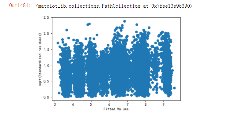
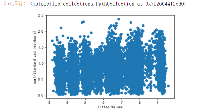
6.5 复杂绘图分析

6.5.1 换一种方法重新验证模型是否符合线性模型

residuals_sq=np.sqrt(abs(residuals_n))
fg3 = fig.add_subplot(223)
fg3.set_title('Scale-Location') 
plt.xlabel('Fitted Values')
plt.ylabel('sqrt(Standardized residuals)')
plt.scatter(y_hat,residuals_sq)

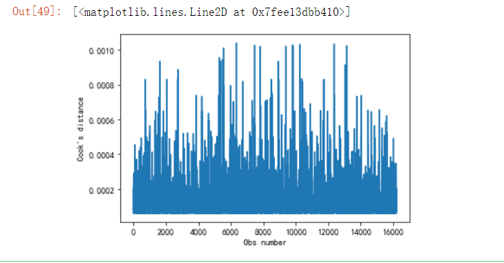
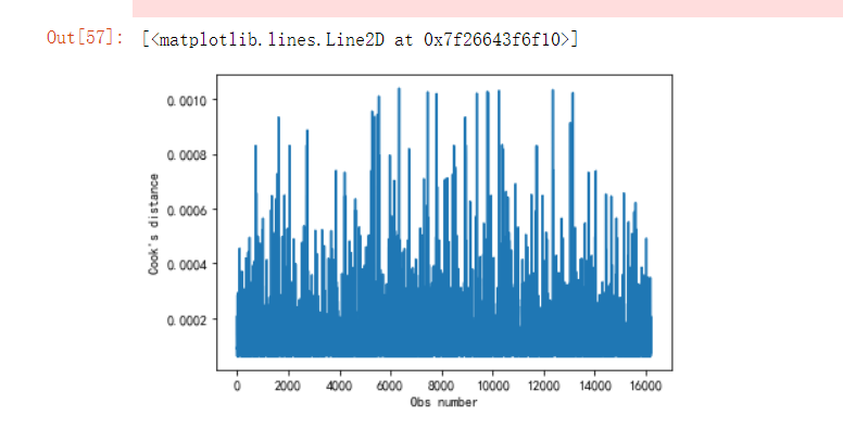
6.5.2 考察样本异常值

n=len(y)
y_m=np.mean(y)
Lyy=np.sum((y-y_m)**2)
Hii=1/n+(y-y_m)**2/Lyy
fg4 = fig.add_subplot(224)  #绘制每个点的库克距离，检测异常点用
fg4.set_title("Cook's distance") 
plt.xlabel('Obs number')
plt.ylabel("Cook's distance")
plt.plot(Hii.tolist())

6.5.3 取对数后重新做以上验证

#对房价取对数，得到——y_log
y_log=df_ana['price'].apply(lambda x:math.log(x))
#对数房价回归模型
model=sm.OLS(y_log,X)
result=model.fit()
result.params

[外链图片转存失败,源站可能有防盗链机制,建议将图片保存下来直接上传(img-uXK94rkO-1629077234162)(Matplotlib基础课程.assets/Matplotlib_09_27.png)]

考察模型参数：

result.summary()

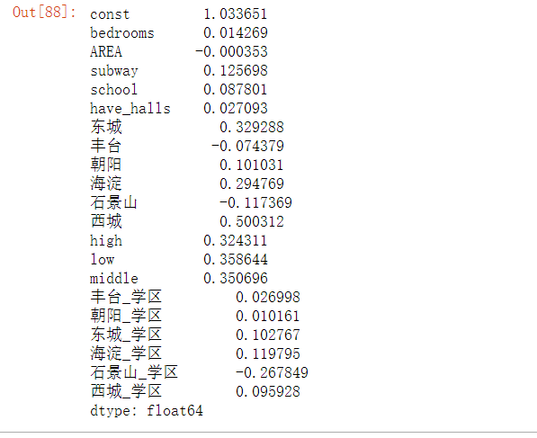
6.5.4 建立新的交叉对数模型

X2=copy.deepcopy(X)

X2['丰台_学区']=X2['丰台']*X2['school']
X2['朝阳_学区']=X2['朝阳']*X2['school']
X2['东城_学区']=X2['东城']*X2['school']
X2['海淀_学区']=X2['海淀']*X2['school']
X2['石景山_学区']=X2['石景山']*X2['school']
X2['西城_学区']=X2['西城']*X2['school']

#对数房价、城区/学区交叉项回归模型
model=sm.OLS(y_log,X2)
result=model.fit()
residus=result.resid
result.params

6.5.5 验证交叉对数模型是否正确

fg = fig.add_subplot(221)
fg.set_title('Residuals VS Fitted') 
plt.xlabel('Fitted Values')
plt.ylabel('Residuals')
plt.scatter(y_hat,residuals)

6.5.6 验证房价是否是正太分布

residuals_n=(residuals-np.mean(residuals))/np.std(residuals)
sorted_=np.sort(residuals_n)
yvals=np.arange(len(sorted_))/float(len(sorted_))
x_label=stats.norm.ppf(yvals)
fg = fig.add_subplot(222)
fg.set_title('Normal Q-Q') 
plt.xlabel('Theoretical Quantiles')
plt.ylabel('Standardized residuals')
plt.scatter(x_label,sorted_)

6.5.7 取平方根，除去符号影响重新验证模型是否符合线性模型

residuals_sq=np.sqrt(abs(residuals_n))
fg3 = fig.add_subplot(223)
fg3.set_title('Scale-Location') 
plt.xlabel('Fitted Values')
plt.ylabel('sqrt(Standardized residuals)')
plt.scatter(y_hat,residuals_sq)

n=len(y)
y_m=np.mean(y)
Lyy=np.sum((y-y_m)**2)
Hii=1/n+(y-y_m)**2/Lyy

fg4 = fig.add_subplot(224)  #绘制每个点的库克距离，检测异常点用
fg4.set_title("Cook's distance") 
plt.xlabel('Obs number')
plt.ylabel("Cook's distance")
plt.plot(Hii.tolist())

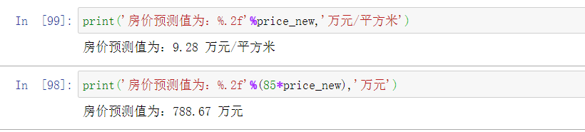
假设需要在西城区买一套临近地铁的学区房，面积85平米。大概需要多少钱。

house_new=[1,2,85,1,1,1,0,0,0,0,0,1,0,1,0,0,0,0,0,0,1]
price_new=np.exp(result.predict(house_new))
#单价
price_new
print('房价预测值为：%.2f'%price_new,'万元/平方米')
print('房价预测值为：%.2f'%(85*price_new),'万元')