资源下载地址：https://download.csdn.net/download/sheziqiong/85601075
资源下载地址：https://download.csdn.net/download/sheziqiong/85601075

• 使用的数据集是 MNIST。
• 完全自己实现神经网络的训练过程，仔细体会了反向传播的流程。

加载数据集

• 这里使用了一个脚本 mnist_loader.py, 将 MNIST 数据集分割为训练集、验证集、测试集。
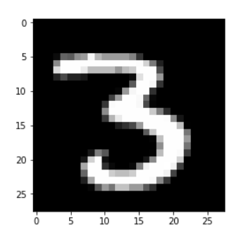
• 展示了其中一幅训练图片，为数字 1.
• 同时，我们也打印出训练集中每个 example 的大小。

# load MNIST data 
training_data, validation_data, test_data = ml.load_data_wrapper()

# show the input data index = 12
x, y = training_data[index]
print(x.shape, y.shape)
plt.imshow(x.reshape((28,28)), 'gray')
(784, 1) (10, 1)





<matplotlib.image.AxesImage at 0x20ebd9607b8>

网络结构与超参数选择

Ex1

• 我们首先尝试的网络结构为：输入层 - 隐含层 - 输出层 （784 - 100 - 10）
• 迭代 20 次，学习率为 0.03，批梯度下降的 batch size 为 100.

# create neural network 
# units of all layers architech = [784, 100, 10]

# iteration numbers num_iter = 20

# learning rate alpha = 0.03

# regularization parameter lambd = 1.2

model = nn.NeuralNetwork(architech, num_iter, alpha, lambd)
# train model 
model.train_model(training_data, test_data=validation_data)

acc = model.evaluate(test_data)
print("Test data acc : {0}".format(acc))
2018-08-10 15:53:08,671: INFO: epoch 0/20 acc : 0.5617
2018-08-10 15:53:20,840: INFO: epoch 2/20 acc : 0.9071
2018-08-10 15:53:32,694: INFO: epoch 4/20 acc : 0.9325
2018-08-10 15:53:44,229: INFO: epoch 6/20 acc : 0.9453
2018-08-10 15:53:55,543: INFO: epoch 8/20 acc : 0.951
2018-08-10 15:54:06,958: INFO: epoch 10/20 acc : 0.9551
2018-08-10 15:54:18,337: INFO: epoch 12/20 acc : 0.9601
2018-08-10 15:54:29,797: INFO: epoch 14/20 acc : 0.9606
2018-08-10 15:54:41,107: INFO: epoch 16/20 acc : 0.962
2018-08-10 15:54:52,640: INFO: epoch 18/20 acc : 0.9626

Test data acc : 0.9583

Ex2

• 将网络结构改为：输入层 - 隐含层 - 输出层 （784 - 64 - 32 - 10）
• 迭代 20 次，学习率为 0.03，批梯度下降的 batch size 为 100.

# create neural network 
# units of all layers architech = [784, 64, 32, 10]

# iteration numbers num_iter = 20

# learning rate alpha = 0.03

# regularization parameter lambd = 1.2

model = nn.NeuralNetwork(architech, num_iter, alpha, lambd)

# train model 
model.train_model(training_data, test_data=validation_data)

acc = model.evaluate(test_data)
print("Test data acc : {0}".format(acc))
2018-08-10 16:02:20,053: INFO: epoch 0/20 acc : 0.8191
2018-08-10 16:02:30,764: INFO: epoch 2/20 acc : 0.9089
2018-08-10 16:02:41,723: INFO: epoch 4/20 acc : 0.9321
2018-08-10 16:02:52,766: INFO: epoch 6/20 acc : 0.9437
2018-08-10 16:03:03,718: INFO: epoch 8/20 acc : 0.953
2018-08-10 16:03:14,544: INFO: epoch 10/20 acc : 0.954
2018-08-10 16:03:26,088: INFO: epoch 12/20 acc : 0.9592
2018-08-10 16:03:38,092: INFO: epoch 14/20 acc : 0.9607
2018-08-10 16:03:49,147: INFO: epoch 16/20 acc : 0.963
2018-08-10 16:03:59,940: INFO: epoch 18/20 acc : 0.9638

Test data acc : 0.959

手写数字识别

• 这里我将自己手写的一串数字作为检测目标，进行分析、识别。
• 基本流程：
  • 1. 图像预处理，如：转换为灰度图像、二值化、形态学操作。
  • 1. 连通域分析，分割出数字部分。
  • 1. 将每个数字图像部分送入上面得到的神经网络模型，得到预测结果。

file_name = 'data\\my_image.jpg'

# read the image image = cv2.imread(file_name, 0)
plt.imshow(image, 'gray')
<matplotlib.image.AxesImage at 0x20ebe352a20>

# binarize _, b_image =  cv2.threshold(image,155,255,cv2.THRESH_BINARY)
b_image = cv2.bitwise_not(b_image) / 255
plt.imshow(b_image, 'gray')
<matplotlib.image.AxesImage at 0x20ebe3b09e8>

# 形态学处理 t_image = cv2.morphologyEx(b_image, cv2.MORPH_OPEN, cv2.getStructuringElement(cv2.MORPH_RECT, (15,15)))
plt.imshow(t_image, 'gray')
<matplotlib.image.AxesImage at 0x20ebe411a90>

分割字符

• 这里使用投影的方法，将图像向水平与垂直两个方向投影（叠加像素）。
• 由下图可以观察到，在图片中，累计像素最多的水平位置与垂直位置正是分割的坐标。
• 如此一来，我们就可以分割出图片中的数字部分。

h, w = t_image.shape

vertical = [np.sum(t_image[:, i]) for i in range(w)]
horizontal = [np.sum(t_image[i, :]) for i in range(h)]

plt.subplot(1,2,1)
plt.title("vertical")
plt.plot(range(w), vertical)

plt.subplot(1,2,2)
plt.title("horizontal")
plt.plot(range(h), horizontal)
[<matplotlib.lines.Line2D at 0x20ec3fa3eb8>]

w_pos = []
h_pos = []
padding = 100
start = 0
for i in range(w-1):
    if vertical[i] == 0 and vertical[i+1] != 0:
        start = i
    elif vertical[i] != 0 and vertical[i+1] == 0:
        w_pos.append((start, (i-start)))

for i in range(h-1):
    if horizontal[i] == 0 and horizontal[i+1] != 0:
        start = i
    elif horizontal[i] != 0 and horizontal[i+1] == 0:
        h_pos.append((start, (i-start)))

img = image
numbers_img = []
raw_img = []
img_size = (28,28)
cnt = len(w_pos)
for i, pos in enumerate(w_pos):
    x, w = pos
    y, h = h_pos[0]
    raw_img.append(image[y:y+h, x:x+w])
    crop_img = cv2.resize(t_image[y-padding:y+padding+h, x-padding:x+padding+w], img_size, interpolation=cv2.INTER_AREA)
    numbers_img.append(crop_img)
    plt.subplot(1,cnt, i+1)
    plt.imshow(crop_img, 'gray')

cnt = len(numbers_img)
for i, num in enumerate(numbers_img):
    y = model.predict(num.reshape([-1, 1]))
    plt.subplot(1,cnt,i+1)
    plt.title("Value : {0}".format(y))
    plt.imshow(raw_img[i], 'gray')
    plt.axis('off')

Summary

1. 在神经网络训练部分，超参数的选择对于模型有着很大的影响。上面实验中使用的参数是我调试了几次后得到的。

2. 在最后手写数字的识别实验部分，一开始识别效果很差。经过检查，发现是裁剪数字部分时，没有在数字四周留出空余部分，导致每次识别效果很差。最后在裁剪时留出了较大的空余部分，得到了很棒的识别效果。

3. Jupyter notebook 真的很棒啊，以前没意识到，现在觉得真滴好用。以后如果给学生留作业的话，很建议用这个。
   y

4. 在神经网络训练部分，超参数的选择对于模型有着很大的影响。上面实验中使用的参数是我调试了几次后得到的。

5. 在最后手写数字的识别实验部分，一开始识别效果很差。经过检查，发现是裁剪数字部分时，没有在数字四周留出空余部分，导致每次识别效果很差。最后在裁剪时留出了较大的空余部分，得到了很棒的识别效果。

6. Jupyter notebook 真的很棒啊，以前没意识到，现在觉得真滴好用。

资源下载地址：https://download.csdn.net/download/sheziqiong/85601075
资源下载地址：https://download.csdn.net/download/sheziqiong/85601075