机器学习-文本处理之电影评论多分类情感分析
背景数据预处理文本分类情感分析
一、背景
文本处理是许多ML应用程序中最常见的任务之一。以下是此类应用的一些示例
- 语言翻译:将句子从一种语言翻译成另一种语言
- 情绪分析:从文本语料库中确定对任何主题或产品等的情绪是积极的、消极的还是中性的
- 垃圾邮件过滤:检测未经请求和不需要的电子邮件/消息。
这些应用程序处理大量文本以执行分类或翻译,并且涉及大量后端工作。将文本转换为算法可以消化的内容是一个复杂的过程。在本文中,我们将讨论文本处理中涉及的步骤。
二、数据预处理
- 分词——将句子转化为词语
- 去除多余的标点符号
- 去除停用词——高频出现的“的、了”之类的词,他们对语义分析没帮助
- 词干提取——通过删除不必要的字符(通常是后缀),将单词缩减为词根。
- 词形还原——通过确定词性并利用语言的详细数据库来消除屈折变化的另一种方法。
我们可以使用python进行许多文本预处理操作。
NLTK(Natural Language Toolkit),自然语言处理工具包,在NLP(自然语言处理)领域中,最常使用的一个Python库。自带语料库,词性分类库。自带分类,分词功能。
分词(Tokenize):word_tokenize生成一个词的列表
import nltk
sentence="I Love China !"
tokens=nltk.word_tokenize(sentence)
tokens
[‘I’, ‘Love’, ‘China’, ‘!’]
中文分词–jieba
>>> import jieba
>>> seg_list=jieba.cut("我正在学习机器学习",cut_all=True)
>>> print("全模式:","/".join(seg_list))
全模式: 我/正在/学习/学习机/机器/学习
>>> seg_list=jieba.cut("我正在学习机器学习",cut_all=False)
>>> print("精确模式:","/".join(seg_list))
精确模式: 我/正在/学习/机器/学习
三、特征提取
在文本处理中,文本中的单词表示离散的、分类的特征。我们如何以算法可以使用的方式对这些数据进行编码?从文本数据到实值向量的映射称为特征提取。用数字表示文本的最简单的技术之一是Bag of Words。
Bag of Words
我们在文本语料库中列出一些独特的单词,称为词汇表。然后我们可以将每个句子或文档表示为一个向量,每个单词表示为1表示现在,0表示不在词汇表中。另一种表示法是计算每个单词在文档中出现的次数。最流行的方法是使用术语频率逆文档频率(TF-IDF)技术。
- Term Frequency (TF)=(术语t出现在•文档中的次数)/(文档中的术语数量)
- Inverse Document Frequency (IDF)=log(N/n),其中,N是文档数量,n是术语t出现在文档中的数量。稀有词的IDF较高,而频繁词的IDF可能较低。因此具有突出显示不同单词的效果。
- 我们计算一个项的TF-IDF值为=TF*IDF

TF('beautiful',Document1) = 2/10, IDF('beautiful')=log(2/2) = 0
TF(‘day’,Document1) = 5/10,  IDF(‘day’)=log(2/1) = 0.30
TF-IDF(‘beautiful’, Document1) = (2/10)*0 = 0
TF-IDF(‘day’, Document1) = (5/10)*0.30 = 0.15
正如您在Document1中看到的,TF-IDF方法严重惩罚了“beautiful”一词,但对“day”赋予了更大的权重。这是由于IDF部分,它为不同的单词赋予了更多的权重。换句话说,从整个语料库的上下文来看,“day”是Document1的一个重要词。Python scikit学习库为文本数据挖掘提供了有效的工具,并提供了计算给定文本语料库的文本词汇表TF-IDF的函数。
使用BOW的一个主要缺点是它放弃了词序,从而忽略了上下文,进而忽略了文档中单词的含义。对于自然语言处理(NLP),保持单词的上下文是至关重要的。为了解决这个问题,我们使用另一种称为单词嵌入的方法。
Word Embedding
它是文本的一种表示形式,其中具有相同含义的单词具有相似的表示形式。换句话说,它表示坐标系中的单词,在坐标系中,基于关系语料库的相关单词被放在更近的位置。
Word2Vec
Word2vec将大量文本作为输入,并生成一个向量空间,每个唯一的单词在该空间中分配一个对应的向量。词向量定位在向量空间中,使得在语料库中共享公共上下文的词在该空间中彼此非常接近。Word2Vec非常擅长捕捉意义,并在诸如计算a到b的类比问题以及c到?的类比问题等任务中演示它?。例如,男人对女人就像叔叔对女人一样?(a)使用基于余弦距离的简单矢量偏移方法。例如,这里有三个单词对的向量偏移量来说明性别关系:
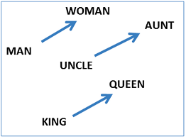
这种向量组合也让我们回答“国王-男人+女人=?”提问并得出结果“女王”!当你认为所有这些知识仅仅来自于在上下文中查看大量单词,而没有提供关于它们的语义的其他信息时,所有这些都是非常值得注意的。
Glove
单词表示的全局向量(GloVe)算法是word2vec方法的扩展,用于有效学习单词向量。glove使用整个文本语料库中的统计信息构建一个显式的单词上下文或单词共现矩阵。结果是一个学习模型,可能会导致更好的单词嵌入。
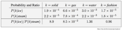
Target words: ice, steam
Probe words: solid, gas, water, fashion
让P(k | w)是单词k出现在单词W的上下文中的概率W.考虑一个与ice有密切关系的词,而不是与steam有关的词,例如solid。P(solid | ice)相对较高,P(solid | steam)相对较低。因此,P(solid | ice)/ P(solid | steam)的比率将很大。如果我们用一个词,比如气体,它与steam有关,但与ice无关,那么P(gas | ice) / P(gas | steam) 的比值就会变小。对于一个既与ice有关又与water有关的词,例如water,我们预计其比率接近1。
单词嵌入将每个单词编码成一个向量,该向量捕获文本语料库中单词之间的某种关系和相似性。这意味着即使是大小写、拼写、标点符号等单词的变体也会自动学习。反过来,这意味着可能不再需要上述一些文本清理步骤。
四、电影评论情感分析实例
根据问题空间和可用数据的不同,有多种方法为各种基于文本的应用程序构建ML模型。
用于垃圾邮件过滤的经典ML方法,如“朴素贝叶斯”或“支持向量机”,已被广泛使用。深度学习技术对于自然语言处理问题(如情感分析和语言翻译)有更好的效果。深度学习模型的训练速度非常慢,并且可以看出,对于简单的文本分类问题,经典的ML方法也能以更快的训练时间给出类似的结果。
让我们使用目前讨论的技术在Kaggle提供的烂番茄电影评论数据集上构建一个情感分析器。
电影评论情感分析

对于电影评论情绪分析,我们将使用Kaggle提供的烂番茄电影评论数据集。在这里,我们根据电影评论的情绪,以五个值为尺度给短语贴上标签:消极的,有些消极的,中性的,有些积极的,积极的。数据集由选项卡分隔的文件组成,其中包含来自数据集的短语ID。每个短语都有一个短语。每个句子都有一个句子ID。重复的短语(如短/常用词)仅在数据中包含一次。情绪标签包括:
- 0 - negative
- 1 - somewhat negative
- 2 - neutral
- 3 - somewhat positive
- 4 - positive
import pandas as pd
import numpy as np
import matplotlib.pyplot as plt
import seaborn as sns
%matplotlib inline
1. 初始化数据
df_train = pd.read_csv("/Users/gawaintan/workSpace/movie-review-sentiment-analysis-kernels-only/train.tsv", sep='\t')
df_train.head()
| PhraseId | SentenceId | Phrase | Sentiment | |
|---|---|---|---|---|
| 0 | 1 | 1 | A series of escapades demonstrating the adage ... | 1 |
| 1 | 2 | 1 | A series of escapades demonstrating the adage ... | 2 |
| 2 | 3 | 1 | A series | 2 |
| 3 | 4 | 1 | A | 2 |
| 4 | 5 | 1 | series | 2 |
df_test = pd.read_csv("/Users/gawaintan/workSpace/movie-review-sentiment-analysis-kernels-only/test.tsv", sep='\t')
df_test.head()
| PhraseId | SentenceId | Phrase | |
|---|---|---|---|
| 0 | 156061 | 8545 | An intermittently pleasing but mostly routine ... |
| 1 | 156062 | 8545 | An intermittently pleasing but mostly routine ... |
| 2 | 156063 | 8545 | An |
| 3 | 156064 | 8545 | intermittently pleasing but mostly routine effort |
| 4 | 156065 | 8545 | intermittently pleasing but mostly routine |
1.1 每个情绪类别中的评论分布
在这里,训练数据集包含了电影评论中占主导地位的中性短语,然后是有些积极的,然后是有些消极的。
df_train.Sentiment.value_counts()
2    79582
3    32927
1    27273
4     9206
0     7072
Name: Sentiment, dtype: int64
df_train.info()
<class 'pandas.core.frame.DataFrame'>
RangeIndex: 156060 entries, 0 to 156059
Data columns (total 4 columns):
 #   Column      Non-Null Count   Dtype
---  ------      --------------   -----
 0   PhraseId    156060 non-null  int64
 1   SentenceId  156060 non-null  int64
 2   Phrase      156060 non-null  object
 3   Sentiment   156060 non-null  int64
dtypes: int64(3), object(1)
memory usage: 4.8+ MB
1.2 删除不重要的列
df_train_1 = df_train.drop(['PhraseId','SentenceId'],axis=1)
df_train_1.head()
| Phrase | Sentiment | |
|---|---|---|
| 0 | A series of escapades demonstrating the adage ... | 1 |
| 1 | A series of escapades demonstrating the adage ... | 2 |
| 2 | A series | 2 |
| 3 | A | 2 |
| 4 | series | 2 |
Let’s check the phrase length of each of the movie reviews.
df_train_1['phrase_len'] = [len(t) for t in df_train_1.Phrase]
df_train_1.head(4)
| Phrase | Sentiment | phrase_len | |
|---|---|---|---|
| 0 | A series of escapades demonstrating the adage ... | 1 | 188 |
| 1 | A series of escapades demonstrating the adage ... | 2 | 77 |
| 2 | A series | 2 | 8 |
| 3 | A | 2 | 1 |
1.3 各情感类别下评论时长的总体分布
fig,ax = plt.subplots(figsize=(5,5))
plt.boxplot(df_train_1.phrase_len)
plt.show()

从上面的箱线图中,有些评论的长度超过 100 个字符。
df_train_1[df_train_1.phrase_len > 100].head()
| Phrase | Sentiment | phrase_len | |
|---|---|---|---|
| 0 | A series of escapades demonstrating the adage ... | 1 | 188 |
| 27 | is also good for the gander , some of which oc... | 2 | 110 |
| 28 | is also good for the gander , some of which oc... | 2 | 108 |
| 116 | A positively thrilling combination of ethnogra... | 3 | 152 |
| 117 | A positively thrilling combination of ethnogra... | 4 | 150 |
df_train_1[df_train_1.phrase_len > 100].loc[0].Phrase
'A series of escapades demonstrating the adage that what is good for the goose is also good for the gander , some of which occasionally amuses but none of which amounts to much of a story .'
1.4 创建负面和正面电影评论的词云
Word Cloud
wordcloud 是文本文件集合中常用词的图形表示。这张图片中每个词的高度是该词在整个文本中出现频率的指标。在进行文本分析时,此类图表非常有用。
1.4.1 筛选出正面和负面的影评
neg_phrases = df_train_1[df_train_1.Sentiment == 0]
neg_words = []
for t in neg_phrases.Phrase:
    neg_words.append(t)
neg_words[:4]
['would have a hard time sitting through this one',
 'have a hard time sitting through this one',
 'Aggressive self-glorification and a manipulative whitewash',
 'self-glorification and a manipulative whitewash']
**pandas.Series.str.cat ** : 使用给定的分隔符连接系列/索引中的字符串。这里我们给一个空格作为分隔符,因此,它将连接每个索引中由空格分隔的所有字符串。
neg_text = pd.Series(neg_words).str.cat(sep=' ')
neg_text[:100]
'would have a hard time sitting through this one have a hard time sitting through this one Aggressive'
for t in neg_phrases.Phrase[:300]:
    if 'good' in t:
        print(t)
's not a particularly good film
covers huge , heavy topics in a bland , surfacey way that does n't offer any insight into why , for instance , good things happen to bad people .
huge , heavy topics in a bland , surfacey way that does n't offer any insight into why , for instance , good things happen to bad people
a bland , surfacey way that does n't offer any insight into why , for instance , good things happen to bad people
所以,我们可以很清楚地看到,即使文本包含“好”这样的词,也是一种负面情绪,因为它表明这部电影不是一部好电影。
pos_phrases = df_train_1[df_train_1.Sentiment == 4] ## 4 is positive sentiment
pos_string = []
for t in pos_phrases.Phrase:
    pos_string.append(t)
pos_text = pd.Series(pos_string).str.cat(sep=' ')
pos_text[:100]
'This quiet , introspective and entertaining independent is worth seeking . quiet , introspective and'
1.4.2 负面分类影评的词云
from wordcloud import WordCloud
wordcloud = WordCloud(width=1600, height=800, max_font_size=200).generate(neg_text)
plt.figure(figsize=(12,10))
plt.imshow(wordcloud, interpolation='bilinear')
plt.axis("off")
plt.show()

一些大的词可以解释得相当中性,例如“film”、“moive”等。我们可以看到一些较小的词在负面电影评论中是有意义的,例如“bad movie”、“dull” 、“boring”等。
然而,在对这部电影的负面分类情绪中,也有一些像“好”这样的词。让我们更深入地了解这些单词/文本:
1.4.3 正分类影评的词云
wordcloud = WordCloud(width=1600, height=800, max_font_size=200).generate(pos_text)
plt.figure(figsize=(12,10))
plt.imshow(wordcloud, interpolation='bilinear')
plt.axis('off')
plt.show()

我再次看到一些大尺寸的中性词,“movie”,“film”,但像“good”,“nest”,“fascinating”这样的正面词也很突出。
1.5 所有5个情感类别的总词频
我们需要 Term Frequency 数据来查看电影评论中使用了哪些词以及使用了多少次。让我们继续使用 CountVectorizer 来计算词频:
from sklearn.feature_extraction.text import CountVectorizer
cvector = CountVectorizer(min_df = 0.0, max_df = 1.0, ngram_range=(1,2))
cvector.fit(df_train_1.Phrase)
CountVectorizer(min_df=0.0, ngram_range=(1, 2))
len(cvector.get_feature_names())
94644
看起来 count vectorizer 已经从语料库中提取了 94644 个单词。可以使用以下代码块获取每个类的词频。
All_matrix=[]
All_words=[]
All_labels=['negative','some-negative','neutral','some-positive','positive']
neg_matrix = cvector.transform(df_train_1[df_train_1.Sentiment == 0].Phrase)
term_freq_df= pd.DataFrame(list(sorted([(word, neg_matrix.sum(axis=0)[0, idx]) for word, idx in cvector.vocabulary_.items()], key = lambda x: x[1], reverse=True)),columns=['Terms','negative'])
term_freq_df=term_freq_df.set_index('Terms')
for i in range(1,5):
    All_matrix.append(cvector.transform(df_train_1[df_train_1.Sentiment == i].Phrase))
    All_words.append(All_matrix[i-1].sum(axis=0))
    aa=pd.DataFrame(list(sorted([(word,All_words[i-1][0, idx]) for word, idx in cvector.vocabulary_.items()], key = lambda x: x[1], reverse=True)),columns=['Terms',All_labels[i]])

    term_freq_df=term_freq_df.join(aa.set_index('Terms'),how='left',lsuffix='_A')


term_freq_df['total'] = term_freq_df['negative'] + term_freq_df['some-negative'] + term_freq_df['neutral'] + term_freq_df['some-positive'] +  term_freq_df['positive']
term_freq_df.sort_values(by='total', ascending=False).head(10)
| negative | some-negative | neutral | some-positive | positive | total | |
|---|---|---|---|---|---|---|
| Terms | ||||||
| the | 3462 | 10885 | 20619 | 12459 | 4208 | 51633 |
| of | 2277 | 6660 | 12287 | 8405 | 3073 | 32702 |
| and | 2549 | 6204 | 10241 | 9180 | 4003 | 32177 |
| to | 1916 | 5571 | 8295 | 5411 | 1568 | 22761 |
| in | 1038 | 2965 | 5562 | 3365 | 1067 | 13997 |
| is | 1372 | 3362 | 3703 | 3489 | 1550 | 13476 |
| that | 1139 | 2982 | 3677 | 3280 | 1260 | 12338 |
| it | 1086 | 3067 | 3791 | 2927 | 863 | 11734 |
| as | 757 | 2184 | 2941 | 2037 | 732 | 8651 |
| with | 452 | 1533 | 2471 | 2365 | 929 | 7750 |
我们可以清楚地看到,像“the”、“in”、“it”等词的频率要高得多,它们对影评的情绪没有任何意义。另一方面,诸如“悲观可笑”之类的词它们在文档中的出现频率非常低,但似乎与电影的情绪有很大关系。
1.6 电影评论分词展示
Next, let’s explore about how different the tokens in two different classes(positive, negative).
from sklearn.feature_extraction.text import CountVectorizer
cvec = CountVectorizer(stop_words='english',max_features=10000)
cvec.fit(df_train_1.Phrase)
CountVectorizer(max_features=10000, stop_words='english')
neg_matrix = cvec.transform(df_train_1[df_train_1.Sentiment == 0].Phrase)
som_neg_matrix = cvec.transform(df_train_1[df_train_1.Sentiment == 1].Phrase)
neu_matrix = cvec.transform(df_train_1[df_train_1.Sentiment == 2].Phrase)
som_pos_matrix = cvec.transform(df_train_1[df_train_1.Sentiment == 3].Phrase)
pos_matrix = cvec.transform(df_train_1[df_train_1.Sentiment == 4].Phrase)

neg_words = neg_matrix.sum(axis=0)
neg_words_freq = [(word, neg_words[0, idx]) for word, idx in cvec.vocabulary_.items()]
neg_tf = pd.DataFrame(list(sorted(neg_words_freq, key = lambda x: x[1], reverse=True)),columns=['Terms','negative'])

neg_tf_df = neg_tf.set_index('Terms')


som_neg_words = som_neg_matrix.sum(axis=0)
som_neg_words_freq = [(word, som_neg_words[0, idx]) for word, idx in cvec.vocabulary_.items()]
som_neg_tf = pd.DataFrame(list(sorted(som_neg_words_freq, key = lambda x: x[1], reverse=True)),columns=['Terms','some-negative'])
som_neg_tf_df = som_neg_tf.set_index('Terms')

neu_words = neu_matrix.sum(axis=0)
neu_words_freq = [(word, neu_words[0, idx]) for word, idx in cvec.vocabulary_.items()]
neu_words_tf = pd.DataFrame(list(sorted(neu_words_freq, key = lambda x: x[1], reverse=True)),columns=['Terms','neutral'])
neu_words_tf_df = neu_words_tf.set_index('Terms')

som_pos_words = som_pos_matrix.sum(axis=0)
som_pos_words_freq = [(word, som_pos_words[0, idx]) for word, idx in cvec.vocabulary_.items()]
som_pos_words_tf = pd.DataFrame(list(sorted(som_pos_words_freq, key = lambda x: x[1], reverse=True)),columns=['Terms','some-positive'])
som_pos_words_tf_df = som_pos_words_tf.set_index('Terms')

pos_words = pos_matrix.sum(axis=0)
pos_words_freq = [(word, pos_words[0, idx]) for word, idx in cvec.vocabulary_.items()]
pos_words_tf = pd.DataFrame(list(sorted(pos_words_freq, key = lambda x: x[1], reverse=True)),columns=['Terms','positive'])
pos_words_tf_df = pos_words_tf.set_index('Terms')

term_freq_df = pd.concat([neg_tf_df,som_neg_tf_df,neu_words_tf_df,som_pos_words_tf_df,pos_words_tf_df],axis=1)

term_freq_df['total'] = term_freq_df['negative'] + term_freq_df['some-negative'] \
                                 + term_freq_df['neutral'] + term_freq_df['some-positive'] \
                                 +  term_freq_df['positive']

term_freq_df.sort_values(by='total', ascending=False).head(15)
| negative | some-negative | neutral | some-positive | positive | total | |
|---|---|---|---|---|---|---|
| Terms | ||||||
| film | 480 | 1281 | 2175 | 1848 | 949 | 6733 |
| movie | 793 | 1463 | 2054 | 1344 | 587 | 6241 |
| like | 332 | 942 | 1167 | 599 | 150 | 3190 |
| story | 153 | 532 | 954 | 664 | 236 | 2539 |
| rrb | 131 | 498 | 1112 | 551 | 146 | 2438 |
| good | 100 | 334 | 519 | 974 | 334 | 2261 |
| lrb | 119 | 452 | 878 | 512 | 137 | 2098 |
| time | 153 | 420 | 752 | 464 | 130 | 1919 |
| characters | 167 | 455 | 614 | 497 | 149 | 1882 |
| comedy | 174 | 341 | 578 | 475 | 245 | 1813 |
| just | 216 | 598 | 550 | 282 | 82 | 1728 |
| life | 77 | 200 | 729 | 544 | 168 | 1718 |
| does | 135 | 566 | 519 | 375 | 79 | 1674 |
| little | 109 | 492 | 580 | 339 | 85 | 1605 |
| funny | 73 | 257 | 267 | 639 | 347 | 1583 |
1.6.1 负面影评中最常用的50个词
y_pos = np.arange(50)
plt.figure(figsize=(12,10))
plt.bar(y_pos, term_freq_df.sort_values(by='negative', ascending=False)['negative'][:50], align='center', alpha=0.5)
plt.xticks(y_pos, term_freq_df.sort_values(by='negative', ascending=False)['negative'][:50].index,rotation='vertical')
plt.ylabel('Frequency')
plt.xlabel('Top 50 negative tokens')
plt.title('Top 50 tokens in negative movie reviews')
Text(0.5, 1.0, 'Top 50 tokens in negative movie reviews')

我们可以看到一些负面词,如“坏”、“最差”、“沉闷”是一些高频词。但是,存在有像“电影”、“电影”、“分钟”这样的中性词支配频率图。
我们再看一下条形图上的前 50 个正面标记
1.6.2 正面影评中最常用的50个词
y_pos = np.arange(50)
plt.figure(figsize=(12,10))
plt.bar(y_pos, term_freq_df.sort_values(by='positive', ascending=False)['positive'][:50], align='center', alpha=0.5)
plt.xticks(y_pos, term_freq_df.sort_values(by='positive', ascending=False)['positive'][:50].index,rotation='vertical')
plt.ylabel('Frequency')
plt.xlabel('Top 50 positive tokens')
plt.title('Top 50 tokens in positive movie reviews')
Text(0.5, 1.0, 'Top 50 tokens in positive movie reviews')
![[外链图片转存失败,源站可能有防盗链机制,建议将图片保存下来直接上传(img-HLxcm1VK-1640793547488)(sentiment-analysis-countvectorizer-tf-idf_files/sentiment-analysis-countvectorizer-tf-idf_51_1.png)]](https://img-blog.csdnimg.cn/ae3848d0b8b64db4bf2b39a52926d2b8.png?x-oss-process=image/watermark,type_d3F5LXplbmhlaQ,shadow_50,text_Q1NETiBAR2F3YWluVGt5,size_20,color_FFFFFF,t_70,g_se,x_16)
Once again, there are some neutral words like “film”, “movie”, are quite high up in the rank.
2. 传统的监督机器学习模型
2.1 特征工程
phrase = np.array(df_train_1['Pfihrase'])
sentiments = np.array(df_train_1['Sentiment'])
# build train and test datasets

from sklearn.model_selection import train_test_split
phrase_train, phrase_test, sentiments_train, sentiments_test = train_test_split(phrase, sentiments, test_size=0.2, random_state=4)
Next, we will try to see how different are the tokens in 4 different classes(positive,some positive,neutral, some negative, negative).
2.2 CountVectorizer & TF-IDF 的实现
2.2.1 CountVectorizer
众所周知,所有机器学习算法都擅长数字;我们必须在不丢失大量信息的情况下将文本数据提取或转换为数字。进行这种转换的一种方法是词袋 (BOW),它为每个词提供一个数字,但效率非常低。因此,一种方法是通过CountVectorizer:它计算文档中的单词数,即将文本文档集合转换为文档中每个单词出现次数的矩阵。
例如:如果我们有如下 3 个文本文档的集合,那么 CountVectorizer 会将其转换为文档中每个单词出现的单独计数,如下所示:
cv1 = CountVectorizer()
x_traincv = cv1.fit_transform(["Hi How are you How are you doing","Hi what's up","Wow that's awesome"])
x_traincv_df = pd.DataFrame(x_traincv.toarray(),columns=list(cv1.get_feature_names()))
x_traincv_df
/Users/gawaintan/miniforge3/lib/python3.9/site-packages/sklearn/utils/deprecation.py:87: FutureWarning: Function get_feature_names is deprecated; get_feature_names is deprecated in 1.0 and will be removed in 1.2. Please use get_feature_names_out instead.
  warnings.warn(msg, category=FutureWarning)
| are | awesome | doing | hi | how | that | up | what | wow | you | |
|---|---|---|---|---|---|---|---|---|---|---|
| 0 | 2 | 0 | 1 | 1 | 2 | 0 | 0 | 0 | 0 | 2 |
| 1 | 0 | 0 | 0 | 1 | 0 | 0 | 1 | 1 | 0 | 0 |
| 2 | 0 | 1 | 0 | 0 | 0 | 1 | 0 | 0 | 1 | 0 |
现在,在 CountVectorizer 的情况下,我们只是在计算文档中的单词数量,很多时候,“are”、“you”、“hi”等单词的数量非常大,这将支配我们的机器学习算法的结果。
2.2.2 TF-IDF 与 CountVectorizer 有何不同?
因此,TF-IDF(代表Term-Frequency-Inverse-Document Frequency)降低了几乎所有文档中出现的常见词的权重,并更加重视出现在文档子集中的词。TF-IDF 的工作原理是通过分配较低的权重来惩罚这些常用词,同时重视特定文档中的一些稀有词。
2.2.3 CountVectorizer参数设置
对于 CountVectorizer 这一次,停用词不会有太大帮助,因为相同的高频词,例如“the”、“to”,在两个类中的出现频率相同。如果这些停用词支配两个类,我将无法获得有意义的结果。因此,我决定删除停用词,并且还将使用 countvectorizer 将 max_features 限制为 10,000。
from sklearn.feature_extraction.text import CountVectorizer, TfidfVectorizer

## Build Bag-Of-Words on train phrases
cv = CountVectorizer(stop_words='english',max_features=10000)
cv_train_features = cv.fit_transform(phrase_train)
# build TFIDF features on train reviews
tv = TfidfVectorizer(min_df=0.0, max_df=1.0, ngram_range=(1,2),
                     sublinear_tf=True)
tv_train_features = tv.fit_transform(phrase_train)
# transform test reviews into features
cv_test_features = cv.transform(phrase_test)
tv_test_features = tv.transform(phrase_test)
print('BOW model:> Train features shape:', cv_train_features.shape, ' Test features shape:', cv_test_features.shape)
print('TFIDF model:> Train features shape:', tv_train_features.shape, ' Test features shape:', tv_test_features.shape)
BOW model:> Train features shape: (124848, 10000)  Test features shape: (31212, 10000)
TFIDF model:> Train features shape: (124848, 93697)  Test features shape: (31212, 93697)
2.3 模型训练、预测和性能评估
####Evaluation metrics


from sklearn import metrics
import numpy as np
import pandas as pd
import matplotlib.pyplot as plt
from sklearn.preprocessing import LabelEncoder
from sklearn.base import clone
from sklearn.preprocessing import label_binarize
from scipy import interp
from sklearn.metrics import roc_curve, auc


def get_metrics(true_labels, predicted_labels):

    print('Accuracy:', np.round(
                        metrics.accuracy_score(true_labels,
                                               predicted_labels),
                        4))
    print('Precision:', np.round(
                        metrics.precision_score(true_labels,
                                               predicted_labels,
                                               average='weighted'),
                        4))
    print('Recall:', np.round(
                        metrics.recall_score(true_labels,
                                               predicted_labels,
                                               average='weighted'),
                        4))
    print('F1 Score:', np.round(
                        metrics.f1_score(true_labels,
                                               predicted_labels,
                                               average='weighted'),
                        4))


def train_predict_model(classifier,
                        train_features, train_labels,
                        test_features, test_labels):
    # build model
    classifier.fit(train_features, train_labels)
    # predict using model
    predictions = classifier.predict(test_features)
    return predictions


def display_confusion_matrix(true_labels, predicted_labels, classes=[1,0]):

    total_classes = len(classes)
    level_labels = [total_classes*[0], list(range(total_classes))]

    cm = metrics.confusion_matrix(y_true=true_labels, y_pred=predicted_labels,
                                  labels=classes)
    cm_frame = pd.DataFrame(data=cm,
                            columns=pd.MultiIndex(levels=[['Predicted:'], classes],
                                                  codes=level_labels),
                            index=pd.MultiIndex(levels=[['Actual:'], classes],
                                                codes=level_labels))
    print(cm_frame)

def display_classification_report(true_labels, predicted_labels, classes=[1,0]):

    report = metrics.classification_report(y_true=true_labels,
                                           y_pred=predicted_labels,
                                           labels=classes)
    print(report)


def display_model_performance_metrics(true_labels, predicted_labels, classes=[1,0]):
    print('Model Performance metrics:')
    print('-'*30)
    get_metrics(true_labels=true_labels, predicted_labels=predicted_labels)
    print('\nModel Classification report:')
    print('-'*30)
    display_classification_report(true_labels=true_labels, predicted_labels=predicted_labels,
                                  classes=classes)
    print('\nPrediction Confusion Matrix:')
    print('-'*30)
    display_confusion_matrix(true_labels=true_labels, predicted_labels=predicted_labels,
                             classes=classes)


def plot_model_decision_surface(clf, train_features, train_labels,
                                plot_step=0.02, cmap=plt.cm.RdYlBu,
                                markers=None, alphas=None, colors=None):

    if train_features.shape[1] != 2:
        raise ValueError("X_train should have exactly 2 columnns!")

    x_min, x_max = train_features[:, 0].min() - plot_step, train_features[:, 0].max() + plot_step
    y_min, y_max = train_features[:, 1].min() - plot_step, train_features[:, 1].max() + plot_step
    xx, yy = np.meshgrid(np.arange(x_min, x_max, plot_step),
                         np.arange(y_min, y_max, plot_step))

    clf_est = clone(clf)
    clf_est.fit(train_features,train_labels)
    if hasattr(clf_est, 'predict_proba'):
        Z = clf_est.predict_proba(np.c_[xx.ravel(), yy.ravel()])[:,1]
    else:
        Z = clf_est.predict(np.c_[xx.ravel(), yy.ravel()])
    Z = Z.reshape(xx.shape)
    cs = plt.contourf(xx, yy, Z, cmap=cmap)

    le = LabelEncoder()
    y_enc = le.fit_transform(train_labels)
    n_classes = len(le.classes_)
    plot_colors = ''.join(colors) if colors else [None] * n_classes
    label_names = le.classes_
    markers = markers if markers else [None] * n_classes
    alphas = alphas if alphas else [None] * n_classes
    for i, color in zip(range(n_classes), plot_colors):
        idx = np.where(y_enc == i)
        plt.scatter(train_features[idx, 0], train_features[idx, 1], c=color,
                    label=label_names[i], cmap=cmap, edgecolors='black',
                    marker=markers[i], alpha=alphas[i])
    plt.legend()
    plt.show()


def plot_model_roc_curve(clf, features, true_labels, label_encoder=None, class_names=None):

    ## Compute ROC curve and ROC area for each class
    fpr = dict()
    tpr = dict()
    roc_auc = dict()
    if hasattr(clf, 'classes_'):
        class_labels = clf.classes_
    elif label_encoder:
        class_labels = label_encoder.classes_
    elif class_names:
        class_labels = class_names
    else:
        raise ValueError('Unable to derive prediction classes, please specify class_names!')
    n_classes = len(class_labels)
    y_test = label_binarize(true_labels, classes=class_labels)
    if n_classes == 2:
        if hasattr(clf, 'predict_proba'):
            prob = clf.predict_proba(features)
            y_score = prob[:, prob.shape[1]-1]
        elif hasattr(clf, 'decision_function'):
            prob = clf.decision_function(features)
            y_score = prob[:, prob.shape[1]-1]
        else:
            raise AttributeError("Estimator doesn't have a probability or confidence scoring system!")

        fpr, tpr, _ = roc_curve(y_test, y_score)
        roc_auc = auc(fpr, tpr)
        plt.plot(fpr, tpr, label='ROC curve (area = {0:0.2f})'
                                 ''.format(roc_auc),
                 linewidth=2.5)

    elif n_classes > 2:
        if hasattr(clf, 'predict_proba'):
            y_score = clf.predict_proba(features)
        elif hasattr(clf, 'decision_function'):
            y_score = clf.decision_function(features)
        else:
            raise AttributeError("Estimator doesn't have a probability or confidence scoring system!")

        for i in range(n_classes):
            fpr[i], tpr[i], _ = roc_curve(y_test[:, i], y_score[:, i])
            roc_auc[i] = auc(fpr[i], tpr[i])

        ## Compute micro-average ROC curve and ROC area
        fpr["micro"], tpr["micro"], _ = roc_curve(y_test.ravel(), y_score.ravel())
        roc_auc["micro"] = auc(fpr["micro"], tpr["micro"])

        ## Compute macro-average ROC curve and ROC area
        # First aggregate all false positive rates
        all_fpr = np.unique(np.concatenate([fpr[i] for i in range(n_classes)]))
        # Then interpolate all ROC curves at this points
        mean_tpr = np.zeros_like(all_fpr)
        for i in range(n_classes):
            mean_tpr += interp(all_fpr, fpr[i], tpr[i])
        # Finally average it and compute AUC
        mean_tpr /= n_classes
        fpr["macro"] = all_fpr
        tpr["macro"] = mean_tpr
        roc_auc["macro"] = auc(fpr["macro"], tpr["macro"])

        ## Plot ROC curves
        plt.figure(figsize=(6, 4))
        plt.plot(fpr["micro"], tpr["micro"],
                 label='micro-average ROC curve (area = {0:0.2f})'
                       ''.format(roc_auc["micro"]), linewidth=3)

        plt.plot(fpr["macro"], tpr["macro"],
                 label='macro-average ROC curve (area = {0:0.2f})'
                       ''.format(roc_auc["macro"]), linewidth=3)

        for i, label in enumerate(class_labels):
            plt.plot(fpr[i], tpr[i], label='ROC curve of class {0} (area = {1:0.2f})'
                                           ''.format(label, roc_auc[i]),
                     linewidth=2, linestyle=':')
    else:
        raise ValueError('Number of classes should be atleast 2 or more')

    plt.plot([0, 1], [0, 1], 'k--')
    plt.xlim([0.0, 1.0])
    plt.ylim([0.0, 1.05])
    plt.xlabel('False Positive Rate')
    plt.ylabel('True Positive Rate')
    plt.title('Receiver Operating Characteristic (ROC) Curve')
    plt.legend(loc="lower right")
    plt.show()
from sklearn.linear_model import SGDClassifier, LogisticRegression

lr = LogisticRegression(penalty='l2', max_iter=100, C=1)
sgd = SGDClassifier(loss='hinge')
2.3.1 CountVectorizer 上的逻辑回归模型
# Logistic Regression model on BOW features
lr_bow_predictions = train_predict_model(classifier=lr,
                                             train_features=cv_train_features, train_labels=sentiments_train,
                                             test_features=cv_test_features, test_labels=sentiments_test)
display_model_performance_metrics(true_labels=sentiments_test, predicted_labels=lr_bow_predictions,
                                      classes=[0,1,2,3,4])
Model Performance metrics:
------------------------------
Accuracy: 0.6369
Precision: 0.6177
Recall: 0.6369
F1 Score: 0.6132

Model Classification report:
------------------------------
              precision    recall  f1-score   support

           0       0.55      0.28      0.37      1426
           1       0.53      0.36      0.43      5428
           2       0.68      0.87      0.77     15995
           3       0.57      0.45      0.50      6603
           4       0.56      0.34      0.42      1760

    accuracy                           0.64     31212
   macro avg       0.58      0.46      0.50     31212
weighted avg       0.62      0.64      0.61     31212


Prediction Confusion Matrix:
------------------------------
          Predicted:
                   0     1      2     3    4
Actual: 0        393   626    349    53    5
        1        251  1967   2936   255   19
        2         57   862  13982  1031   63
        3         15   236   3023  2941  388
        4          1    23    253   888  595
2.3.2 基于 TF-IDF 特征的逻辑回归模型
# Logistic Regression model on TF-IDF features
lr_tfidf_predictions = train_predict_model(classifier=lr,
                                               train_features=tv_train_features, train_labels=sentiments_train,
                                               test_features=tv_test_features, test_labels=sentiments_test)
display_model_performance_metrics(true_labels=sentiments_test, predicted_labels=lr_tfidf_predictions,
                                      classes=[0,1,2,3,4])
Model Performance metrics:
------------------------------
Accuracy: 0.6455
Precision: 0.6314
Recall: 0.6455
F1 Score: 0.6189

Model Classification report:
------------------------------
              precision    recall  f1-score   support

           0       0.60      0.22      0.32      1426
           1       0.56      0.38      0.45      5428
           2       0.67      0.89      0.77     15995
           3       0.60      0.47      0.53      6603
           4       0.60      0.29      0.39      1760

    accuracy                           0.65     31212
   macro avg       0.61      0.45      0.49     31212
weighted avg       0.63      0.65      0.62     31212


Prediction Confusion Matrix:
------------------------------
          Predicted:
                   0     1      2     3    4
Actual: 0        312   681    408    22    3
        1        177  2051   3066   125    9
        2         29   793  14193   944   36
        3          2   109   3115  3088  289
        4          0     9    281   966  504
2.3.3 基于Countvectorizer的SGD模型
# SGD model on Countvectorizer
sgd_bow_predictions = train_predict_model(classifier=sgd,
                                             train_features=cv_train_features, train_labels=sentiments_train,
                                             test_features=cv_test_features, test_labels=sentiments_test)
display_model_performance_metrics(true_labels=sentiments_test, predicted_labels=sgd_bow_predictions,
                                      classes=[0,1,2,3,4])
Model Performance metrics:
------------------------------
Accuracy: 0.5988
Precision: 0.5776
Recall: 0.5988
F1 Score: 0.5455

Model Classification report:
------------------------------
              precision    recall  f1-score   support

           0       0.52      0.23      0.32      1426
           1       0.54      0.19      0.28      5428
           2       0.62      0.93      0.74     15995
           3       0.54      0.30      0.38      6603
           4       0.52      0.29      0.37      1760

    accuracy                           0.60     31212
   macro avg       0.55      0.39      0.42     31212
weighted avg       0.58      0.60      0.55     31212


Prediction Confusion Matrix:
------------------------------
          Predicted:
                   0     1      2     3    4
Actual: 0        332   392    646    49    7
        1        234  1025   3909   230   30
        2         56   371  14874   637   57
        3         18   106   4156  1956  367
        4          4    15    502   735  504
2.3.4 基于TF-IDF的SGD模型
# SGD model on TF-IDF
sgd_tfidf_predictions = train_predict_model(classifier=sgd,
                                                train_features=tv_train_features, train_labels=sentiments_train,
                                                test_features=tv_test_features, test_labels=sentiments_test)
display_model_performance_metrics(true_labels=sentiments_test, predicted_labels=sgd_tfidf_predictions,
                                      classes=[0,1,2,3,4])
Model Performance metrics:
------------------------------
Accuracy: 0.5594
Precision: 0.5543
Recall: 0.5594
F1 Score: 0.4666

Model Classification report:
------------------------------
              precision    recall  f1-score   support

           0       0.60      0.11      0.18      1426
           1       0.52      0.09      0.16      5428
           2       0.56      0.97      0.71     15995
           3       0.55      0.16      0.25      6603
           4       0.59      0.15      0.24      1760

    accuracy                           0.56     31212
   macro avg       0.56      0.30      0.31     31212
weighted avg       0.55      0.56      0.47     31212


Prediction Confusion Matrix:
------------------------------
          Predicted:
                   0    1      2     3    4
Actual: 0        152  241   1020    13    0
        1         83  512   4759    67    7
        2         17  193  15447   315   23
        3          2   38   5328  1085  150
        4          0    2    993   502  263
2.3.5 基于TF-IDF的随机森林模型
from sklearn.ensemble import RandomForestClassifier
rfc = RandomForestClassifier(n_jobs=-1)
# RandomForest model on TF-IDF
rfc_tfidf_predictions = train_predict_model(classifier=rfc,
                                                train_features=tv_train_features, train_labels=sentiments_train,
                                                test_features=tv_test_features, test_labels=sentiments_test)
display_model_performance_metrics(true_labels=sentiments_test, predicted_labels=rfc_tfidf_predictions,
                                      classes=[0,1,2,3,4])
Model Performance metrics:
------------------------------
Accuracy: 0.6423
Precision: 0.6267
Recall: 0.6423
F1 Score: 0.6274

Model Classification report:
------------------------------
              precision    recall  f1-score   support

           0       0.47      0.36      0.41      1426
           1       0.56      0.42      0.48      5428
           2       0.70      0.84      0.76     15995
           3       0.58      0.46      0.51      6603
           4       0.50      0.40      0.45      1760

    accuracy                           0.64     31212
   macro avg       0.56      0.50      0.52     31212
weighted avg       0.63      0.64      0.63     31212


Prediction Confusion Matrix:
------------------------------
          Predicted:
                   0     1      2     3    4
Actual: 0        520   605    283    17    1
        1        465  2281   2539   133   10
        2        101  1094  13479  1258   63
        3          8   115   2793  3057  630
        4          2     6    217   825  710
基于TF-IDF的逻辑回归模型优于其他机器学习算法.

为开发者提供学习成长、分享交流、生态实践、资源工具等服务,帮助开发者快速成长。
更多推荐


 19
19 0
0- 0


 已为社区贡献1条内容

所有评论(0)