实验环境:

1. Pytorch 1.7.0
2. torchvision 0.8.2
3. Python 3.8
4. CUDA10.2 + cuDNN v7.6.5
5. Win10 + Pycharm
6. GTX1660, 6G

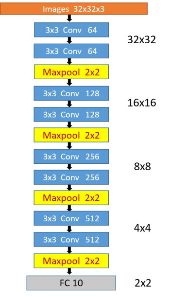
网络结构采用最简洁的类VGG结构，即全部由3*3卷积和最大池化组成，后面接一个全连接层用于分类，网络大小仅18M左右。

神经网络结构图：

Pytorch上搭建网络：

class Block(nn.Module):
    def __init__(self, inchannel, outchannel, res=True):
        super(Block, self).__init__()
        self.res = res     # 是否带残差连接
        self.left = nn.Sequential(
            nn.Conv2d(inchannel, outchannel, kernel_size=3, padding=1, bias=False),
            nn.BatchNorm2d(outchannel),
            nn.ReLU(inplace=True),
            nn.Conv2d(outchannel, outchannel, kernel_size=3, padding=1, bias=False),
            nn.BatchNorm2d(outchannel),
        )
        if stride != 1 or inchannel != outchannel:
            self.shortcut = nn.Sequential(
                nn.Conv2d(inchannel, outchannel, kernel_size=1, bias=False),
                nn.BatchNorm2d(outchannel),
            )
        else:
            self.shortcut = nn.Sequential()

        self.relu = nn.Sequential(
            nn.ReLU(inplace=True),
        )

    def forward(self, x):
        out = self.left(x)
        if self.res:
            out += self.shortcut(x)
        out = self.relu(out)
        return out


class myModel(nn.Module):
    def __init__(self, cfg=[64, 'M', 128,  'M', 256, 'M', 512, 'M'], res=True):
        super(myModel, self).__init__()
        self.res = res       # 是否带残差连接
        self.cfg = cfg       # 配置列表
        self.inchannel = 3   # 初始输入通道数
        self.futures = self.make_layer()
        # 构建卷积层之后的全连接层以及分类器：
        self.classifier = nn.Sequential(nn.Dropout(0.4),            # 两层fc效果还差一些
                                        nn.Linear(4 * 512, 10), )   # fc，最终Cifar10输出是10类

    def make_layer(self):
        layers = []
        for v in self.cfg:
            if v == 'M':
                layers.append(nn.MaxPool2d(kernel_size=2, stride=2))
            else:
                layers.append(Block(self.inchannel, v, self.res))
                self.inchannel = v    # 输入通道数改为上一层的输出通道数
        return nn.Sequential(*layers)

    def forward(self, x):
        out = self.futures(x)
        # view(out.size(0), -1): change tensor size from (N ,H , W) to (N, H*W)
        out = out.view(out.size(0), -1)
        out = self.classifier(out)
        return out

该网络可以很方便的改造成带残差的，只要在初始化网络时，将参数res设为True即可，并可改变cfg配置列表来方便的修改网络层数。

Pytorch上训练：

所选数据集为Cifar-10，该数据集共有60000张带标签的彩色图像，这些图像尺寸32*32，分为10个类，每类6000张图。这里面有50000张用于训练，每个类5000张，另外10000用于测试，每个类1000张。
训练策略如下：

1. 优化器：momentum=0.9 的 optim.SGD，adam在很多情况下能加速收敛，但因为是自适应学习率，在训练后期存在不能收敛到全局极值点的问题，所以采用能手动调节学习率的SGD，现在很多比赛和论文中也是采用该策略。设置weight_decay=5e-3，即设置较大的L2正则来降低过拟合。

# 定义损失函数和优化器
loss_func = nn.CrossEntropyLoss()
optimizer = optim.SGD(model.parameters(), lr=LR, momentum=0.9, weight_decay=5e-3)

2. 学习率：optim.lr_scheduler.MultiStepLR，参数设为：milestones=[int(num_epochs * 0.56), int(num_epochs * 0.78)], gamma=0.1，即在0.56倍epochs和0.78时分别下降为前一阶段学习率的0.1倍。

# 学习率调整策略 MultiStep：
scheduler = optim.lr_scheduler.MultiStepLR(optimizer=optimizer,
                   milestones=[int(num_epochs * 0.56), int(num_epochs * 0.78)],
                   gamma=0.1, last_epoch=-1)

在每个epoch训练完的时候一定要记得step一下，不然不会更新学习率，可以通过get_last_lr()来查看最新的学习率

# 更新学习率并查看当前学习率
scheduler.step()
print('\t last_lr:', scheduler.get_last_lr())

3. 数据策略：
   实验表明，针对cifar10数据集，随机水平翻转、随机遮挡、随机中心裁剪能有效提高验证集准确率，而旋转、颜色抖动等则无效。

     norm_mean = [0.485, 0.456, 0.406]      # 均值
     norm_std = [0.229, 0.224, 0.225]       # 方差      
     transforms.Normalize(norm_mean, norm_std),                    #将[0,1]归一化到[-1,1]
     transforms.RandomHorizontalFlip(),                            # 随机水平镜像
     transforms.RandomErasing(scale=(0.04, 0.2), ratio=(0.5, 2)),  # 随机遮挡
     transforms.RandomCrop(32, padding=4)                          # 随机中心裁剪

4. 超参数：

batch_size = 512     # 约占用显存4G
num_epochs = 200     # 训练轮数
LR = 0.01            # 初始学习率    

实验结果：best_acc= 94.71%

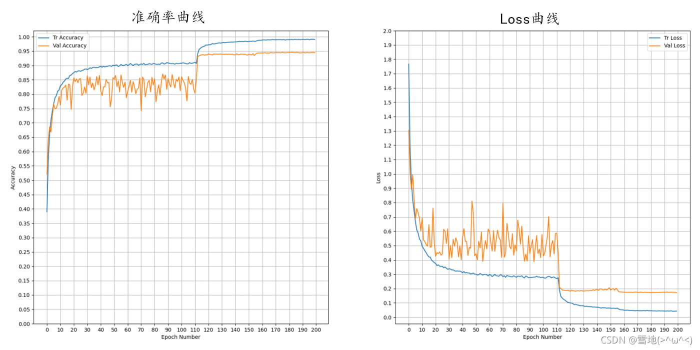
另外，将网络改成14层的带残差结构后，准确率上升到了95.56%，但是网络大小也从18M到了43M。以下是14层残差网络的全部代码，8层的只需修改cfg和初始化时的res参数：
cfg=[64, ‘M’, 128, 128, ‘M’, 256, 256, ‘M’, 512, 512,‘M’] 修改为 [64, ‘M’, 128, ‘M’, 256, ‘M’, 512, ‘M’]

# *_* coding : UTF-8 *_*
# 开发人员： csu·pan-_-||
# 开发时间： 2020/12/29 15:17
# 文件名称： battey_class.py
# 开发工具： PyCharm
# 功能描述： 自建CNN对cifar10进行分类

import torch
from torchvision import datasets, transforms
import torch.nn as nn
import torch.optim as optim
from torch.utils.data import DataLoader
import onnx
import time
import numpy as np
import matplotlib.pyplot as plt


class Block(nn.Module):
    def __init__(self, inchannel, outchannel, res=True, stride=1):
        super(Block, self).__init__()
        self.res = res     # 是否带残差连接
        self.left = nn.Sequential(
            nn.Conv2d(inchannel, outchannel, kernel_size=3, padding=1, stride=stride, bias=False),
            nn.BatchNorm2d(outchannel),
            nn.ReLU(inplace=True),
            nn.Conv2d(outchannel, outchannel, kernel_size=3, padding=1, stride=1, bias=False),
            nn.BatchNorm2d(outchannel),
        )
        if stride != 1 or inchannel != outchannel:
            self.shortcut = nn.Sequential(
                nn.Conv2d(inchannel, outchannel, kernel_size=1, bias=False),
                nn.BatchNorm2d(outchannel),
            )
        else:
            self.shortcut = nn.Sequential()

        self.relu = nn.Sequential(
            nn.ReLU(inplace=True),
        )

    def forward(self, x):
        out = self.left(x)
        if self.res:
            out += self.shortcut(x)
        out = self.relu(out)
        return out


class myModel(nn.Module):
    def __init__(self, cfg=[64, 'M', 128, 128, 'M', 256, 256, 'M', 512, 512,'M'], res=True):
        super(myModel, self).__init__()
        self.res = res       # 是否带残差连接
        self.cfg = cfg       # 配置列表
        self.inchannel = 3   # 初始输入通道数
        self.futures = self.make_layer()
        # 构建卷积层之后的全连接层以及分类器：
        self.classifier = nn.Sequential(nn.Dropout(0.4),           # 两层fc效果还差一些
                                        nn.Linear(4 * 512, 10), )   # fc，最终Cifar10输出是10类

    def make_layer(self):
        layers = []
        for v in self.cfg:
            if v == 'M':
                layers.append(nn.MaxPool2d(kernel_size=2, stride=2))
            else:
                layers.append(Block(self.inchannel, v, self.res))
                self.inchannel = v    # 输入通道数改为上一层的输出通道数
        return nn.Sequential(*layers)

    def forward(self, x):
        out = self.futures(x)
        # view(out.size(0), -1): change tensor size from (N ,H , W) to (N, H*W)
        out = out.view(out.size(0), -1)
        out = self.classifier(out)
        return out

all_start = time.time()
# 使用torchvision可以很方便地下载Cifar10数据集，而torchvision下载的数据集为[0,1]的PILImage格式
# 我们需要将张量Tensor归一化到[-1,1]
norm_mean = [0.485, 0.456, 0.406]  # 均值
norm_std = [0.229, 0.224, 0.225]  # 方差
transform_train = transforms.Compose([transforms.ToTensor(),  # 将PILImage转换为张量
                                      # 将[0,1]归一化到[-1,1]
                                      transforms.Normalize(norm_mean, norm_std),
                                      transforms.RandomHorizontalFlip(),  # 随机水平镜像
                                      transforms.RandomErasing(scale=(0.04, 0.2), ratio=(0.5, 2)),  # 随机遮挡
                                      transforms.RandomCrop(32, padding=4)  # 随机中心裁剪
                                      ])

transform_test = transforms.Compose([transforms.ToTensor(),
                                     transforms.Normalize(norm_mean, norm_std)])

# 超参数：
batch_size = 256
num_epochs = 200   # 训练轮数
LR = 0.01          # 初始学习率

# 选择数据集:
trainset = datasets.CIFAR10(root='Datasets', train=True, download=True, transform=transform_train)
testset = datasets.CIFAR10(root='Datasets', train=False, download=True, transform=transform_test)
# 加载数据:
train_data = DataLoader(dataset=trainset, batch_size=batch_size, shuffle=True)
valid_data = DataLoader(dataset=testset, batch_size=batch_size, shuffle=False)
cifar10_classes = ('plane', 'car', 'bird', 'cat', 'deer', 'dog', 'frog', 'horse', 'ship', 'truck')

train_data_size = len(trainset)
valid_data_size = len(testset)

print('train_size: {:4d}  valid_size:{:4d}'.format(train_data_size, valid_data_size))

device = torch.device("cuda:0" if torch.cuda.is_available() else "cpu")

model = myModel(res=True)

# 定义损失函数和优化器
loss_func = nn.CrossEntropyLoss()
optimizer = optim.SGD(model.parameters(), lr=LR, momentum=0.9, weight_decay=5e-3)

# 学习率调整策略 MultiStep：
scheduler = optim.lr_scheduler.MultiStepLR(optimizer=optimizer,
                                           milestones=[int(num_epochs * 0.56), int(num_epochs * 0.78)],
                                           gamma=0.1, last_epoch=-1)

# 训练和验证：
def train_and_valid(model, loss_function, optimizer, epochs=10):
    model.to(device)
    history = []
    best_acc = 0.0
    best_epoch = 0

    for epoch in range(epochs):
        epoch_start = time.time()
        print("Epoch: {}/{}".format(epoch + 1, epochs))

        model.train()

        train_loss = 0.0
        train_acc = 0.0
        valid_loss = 0.0
        valid_acc = 0.0

        for i, (inputs, labels) in enumerate(train_data):
            inputs = inputs.to(device)
            labels = labels.to(device)

            # 因为这里梯度是累加的，所以每次记得清零
            optimizer.zero_grad()

            outputs = model(inputs)

            loss = loss_function(outputs, labels)

            loss.backward()

            optimizer.step()

            train_loss += loss.item() * inputs.size(0)

            ret, predictions = torch.max(outputs.data, 1)
            correct_counts = predictions.eq(labels.data.view_as(predictions))

            acc = torch.mean(correct_counts.type(torch.FloatTensor))

            train_acc += acc.item() * inputs.size(0)

        with torch.no_grad():
            model.eval()

            for j, (inputs, labels) in enumerate(valid_data):
                inputs = inputs.to(device)
                labels = labels.to(device)

                outputs = model(inputs)

                loss = loss_function(outputs, labels)

                valid_loss += loss.item() * inputs.size(0)

                ret, predictions = torch.max(outputs.data, 1)
                correct_counts = predictions.eq(labels.data.view_as(predictions))

                acc = torch.mean(correct_counts.type(torch.FloatTensor))

                valid_acc += acc.item() * inputs.size(0)
        # 更新学习率并查看当前学习率
        scheduler.step()
        print('\t last_lr:', scheduler.get_last_lr())

        avg_train_loss = train_loss / train_data_size
        avg_train_acc = train_acc / train_data_size

        avg_valid_loss = valid_loss / valid_data_size
        avg_valid_acc = valid_acc / valid_data_size

        history.append([avg_train_loss, avg_valid_loss, avg_train_acc, avg_valid_acc])

        if best_acc < avg_valid_acc:
            best_acc = avg_valid_acc
            best_epoch = epoch + 1

        epoch_end = time.time()

        print(
            "\t Training: Loss: {:.4f}, Accuracy: {:.4f}%, "
            "\n\t Validation: Loss: {:.4f}, Accuracy: {:.4f}%, Time: {:.3f}s".format(
                avg_train_loss, avg_train_acc * 100, avg_valid_loss, avg_valid_acc * 100,
                                epoch_end - epoch_start
            ))
        print("\t Best Accuracy for validation : {:.4f} at epoch {:03d}".format(best_acc, best_epoch))

        torch.save(model, '%s/' % 'cifar10_my' + '%02d' % (epoch + 1) + '.pt')  # 保存模型

        # # 存储模型为onnx格式：
        # d_cuda = torch.rand(1, 3, 32, 32, dtype=torch.float).to(device='cuda')
        # onnx_path = '%s/' % 'cifar10_shuffle' + '%02d' % (epoch + 1) + '.onnx'
        # torch.onnx.export(model.to('cuda'), d_cuda, onnx_path)
        # shape_path = '%s/' % 'cifar10_shuffle' + '%02d' % (epoch + 1) + '_shape.onnx'
        # onnx.save(onnx.shape_inference.infer_shapes(onnx.load(onnx_path)), shape_path)
        # print('\t export shape success...')

    return model, history


trained_model, history = train_and_valid(model, loss_func, optimizer, num_epochs)

history = np.array(history)
# Loss曲线
plt.figure(figsize=(10, 10))
plt.plot(history[:, 0:2])
plt.legend(['Tr Loss', 'Val Loss'])
plt.xlabel('Epoch Number')
plt.ylabel('Loss')
# 设置坐标轴刻度
plt.xticks(np.arange(0, num_epochs + 1, step=10))
plt.yticks(np.arange(0, 2.05, 0.1))
plt.grid()  # 画出网格
plt.savefig('cifar10_shuffle_' + '_loss_curve1.png')

# 精度曲线
plt.figure(figsize=(10, 10))
plt.plot(history[:, 2:4])
plt.legend(['Tr Accuracy', 'Val Accuracy'])
plt.xlabel('Epoch Number')
plt.ylabel('Accuracy')
# 设置坐标轴刻度
plt.xticks(np.arange(0, num_epochs + 1, step=10))
plt.yticks(np.arange(0, 1.05, 0.05))
plt.grid()  # 画出网格
plt.savefig('cifar10_shuffle_' + '_accuracy_curve1.png')

all_end = time.time()
all_time = round(all_end - all_start)
print('all time: ', all_time, ' 秒')
print("All Time: {:d} 分 {:d} 秒".format(all_time // 60, all_time % 60))