深度学习实际—手写体识别

本文介绍机器学习中的一个实例-手写体识别。

zaiziwamei

3777人浏览 · 2022-10-06 23:15:22

zaiziwamei · 2022-10-06 23:15:22 发布

前言

本文介绍机器学习中的一个实例-手写体识别。

1. 什么是机器识别手写数字？

即输入一张手写体0-9的数字，计算机自动识别数字并给出结果。

2. MNIST数据集是什么？

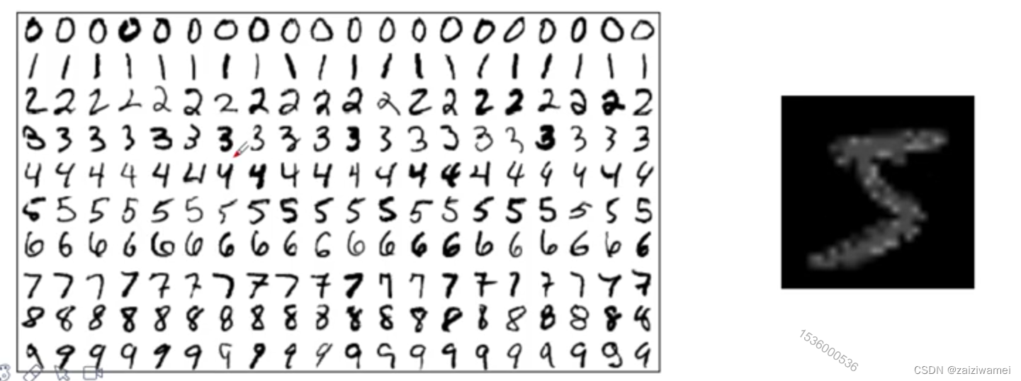
此数据集为手写体数字。
该数据集包含60,000个用于训练的示例和10,000个用于测试的示例。
数据集包含了0-9共10类手写数字图片，每张图片都做了尺寸归一化，都是28x28大小的灰度图。

在这里插入图片描述

3. 显示MNIST数据集

可通过加载数据集在TensorBoard界面加载数据集，代码如下：

# 1 加载包
from torchvision import datasets,transforms
from torch.utils.data import DataLoader
from torch.utils.tensorboard import SummaryWriter  # 加载图像的包

# 2 构建pipeline,对图像做处理
pipeline = transforms.Compose([
    transforms.ToTensor(),  # 将图片转换成tensor
])
# 3 下载数据集
train_set = datasets.MNIST("data",train=True, download=True, transform=pipeline)

# 4 加载数据
train_loader = DataLoader(train_set, batch_size=1, shuffle=True)  # shuffle=True,将数据集打乱
img,target = train_set[0]

# 5 数据展示

# 5.1 测试数据集中第一张图片
print(img.shape)
print(target)

# 5.2 TensorBoard界面显示数据
writer = SummaryWriter("dataloader_show")
step = 0
for data in train_loader:
    imgs, targets = data
    writer.add_images("train_data", imgs, step)
    step = step + 1
writer.close()
# cd "D:\document\document\major_study\Machine-Learning\实践项目\"
# tensorboard --logdir=dataloader_show --port=6007 #更换通道位置打开

输出：
torch.Size([1, 28, 28])
5

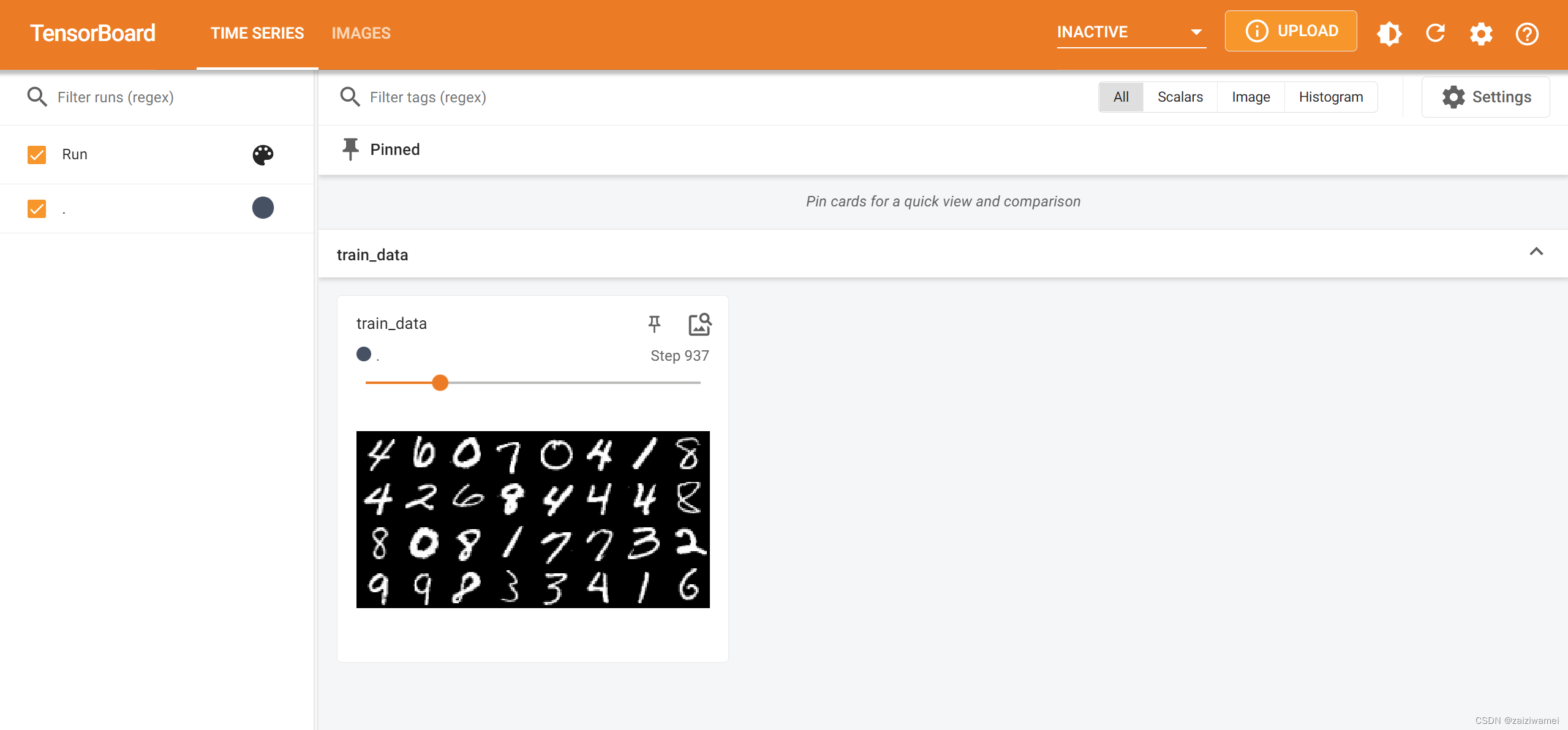
在pycharm的Terminal通道选择Command Prompt界面
并输入：

 tensorboard --logdir=dataloader_show --port=6007

获得的如下界面，从而展示了图像
在这里插入图片描述

4. 名词解释

4. 1 图像

图像在计算机中表示方式有多种，图像在计算机中以像素点集合的形式存在，每个像素点由三通道组成，每个通道用0-255数值表示。本文采用的MINIST数据集中的手写体只有一个通道到，像素为28×28。

4. 2 卷积层

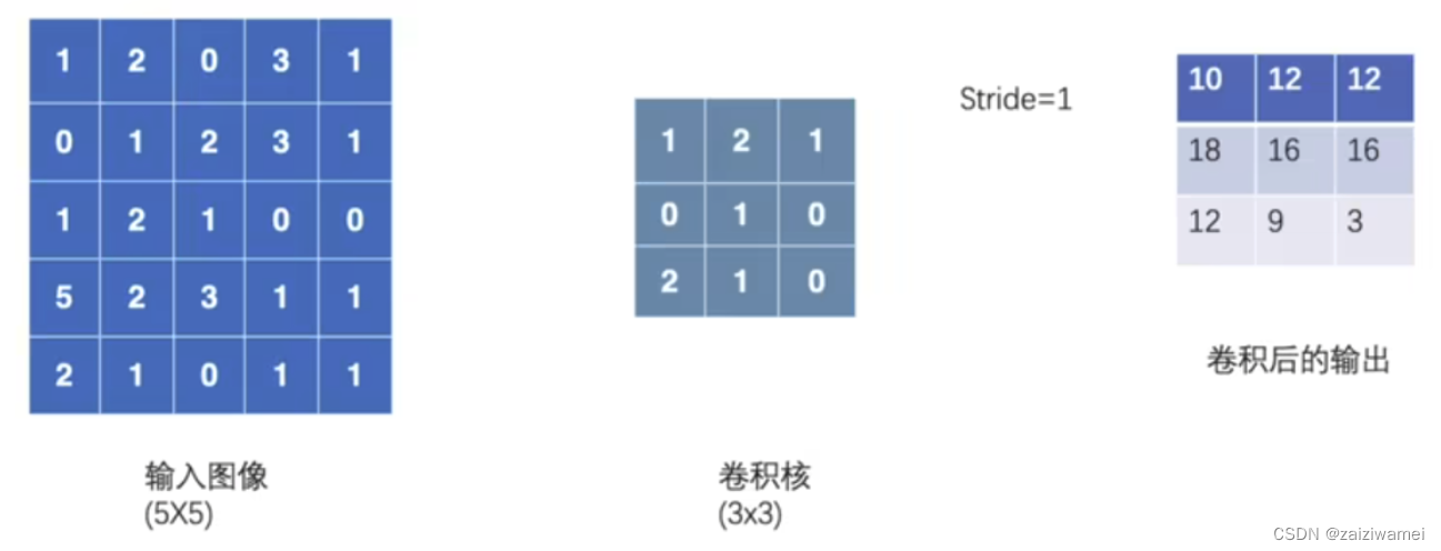在这里插入图片描述卷积层的作用是提取一个局部区域的特征，不同的卷积核相当于不同的特征提取器移动，提取图像特称。

4. 3 池化层

在这里插入图片描述
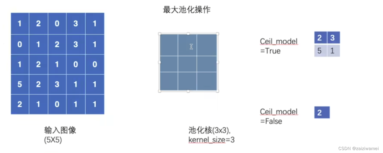
池化层的作用是进行特征选择，降低特征数量，从而减少参数数量。常用池化方法由最大池化和平均池化。

4. 4 线性层

本文为将三维矩阵拉平为一维度向量，也即将卷积或池化层拉平为线性层。、

4. 5 激活函数

含义：激活函数是人工神经网络的神经元上运行的函数。

作用：
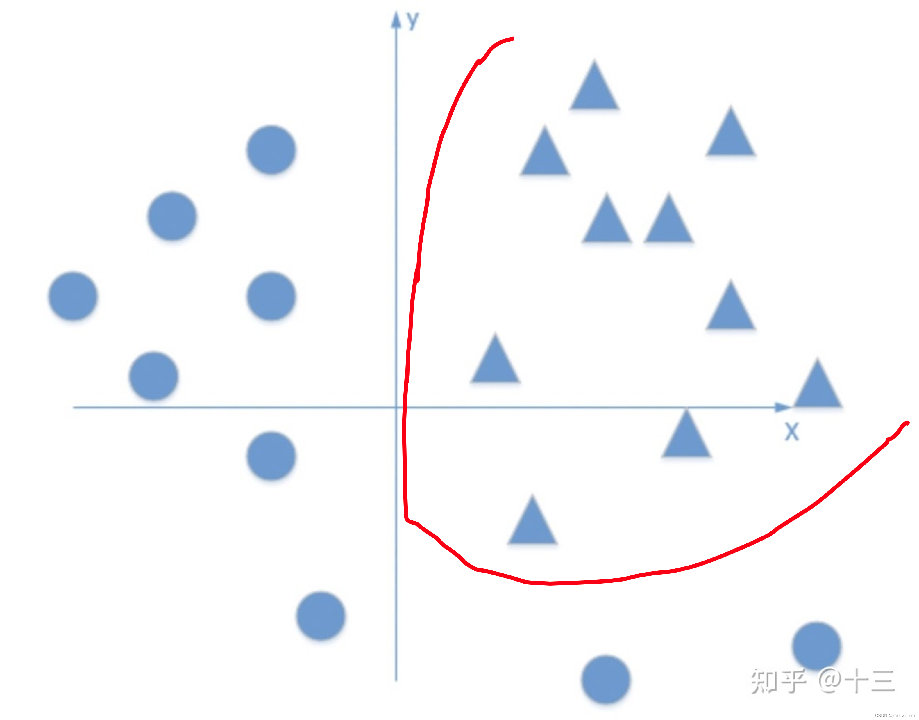
如果不用激活函数，每一层输出都是上层输入的线性函数，无论神经网络有多少层，输出都是输入的线性组合，这种情况就是最原始的感知机，这无法模拟某些非线性情况。激活函数的使用给神经元引入了非线性因素，使得神经网络可以任意逼近任何非线性函数，这样神经网络就可以应用到众多的非线性模型中。

如下图所示，多层感知机+激活函数得到的曲线有可能把三角和圆分开。
在这里插入图片描述
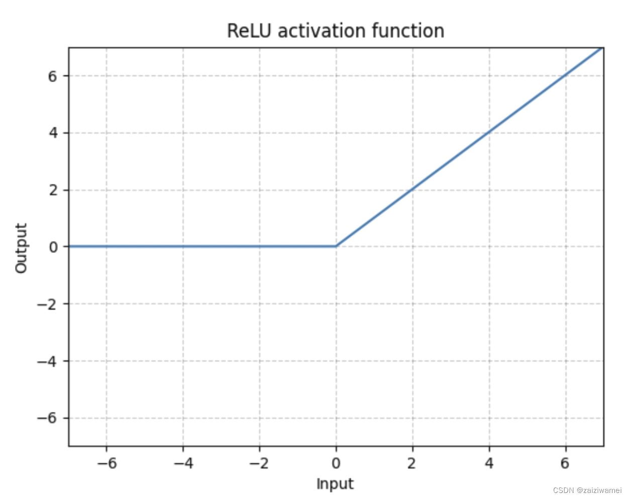
常用的激活函数：Sigmoid函数、Tanh函数、ReLU函数，其中Sigmoid函数可以将较大范围内变化的输入挤压到(0,1)输出。ReLU函数表达式与图像如下图所示。

在这里插入图片描述

在这里插入图片描述应用：本文每进行一次卷积、池化、拉平或连接（除最好一次）操作后都要进行一次ReLU激活操作。最有一次连接操作后使用了Sigmoid激活函数来压缩输出范围。
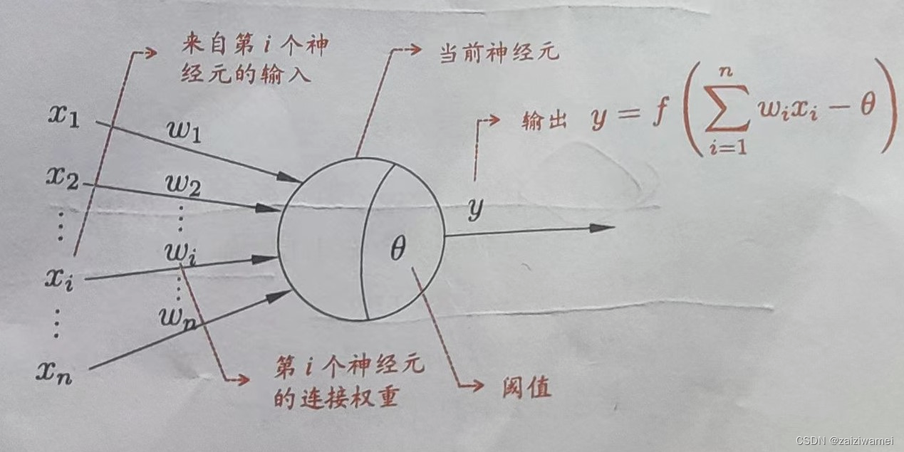
连接层中的激活函数：如下图所示，单神经元中为激活函数f，其使用将连接层中数据非线性化。
在这里插入图片描述 卷积层中的激活函数：本质上卷积也是一种线性放射变换，引入激活函数自然是为了非线性化。

4. 6 损失函数

含义：计算实际输出和目标之间的差距
交叉熵损失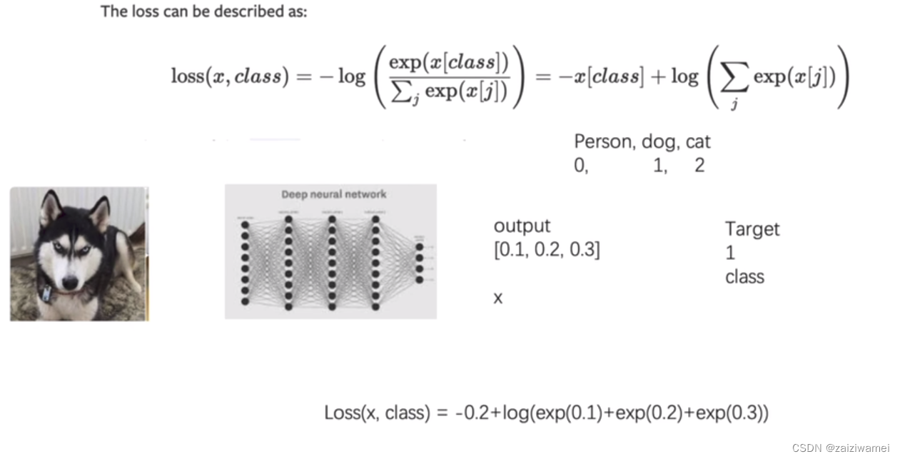：在这里插入图片描述

4.7 正则化

模型出现过拟合时，降低模型复杂度。

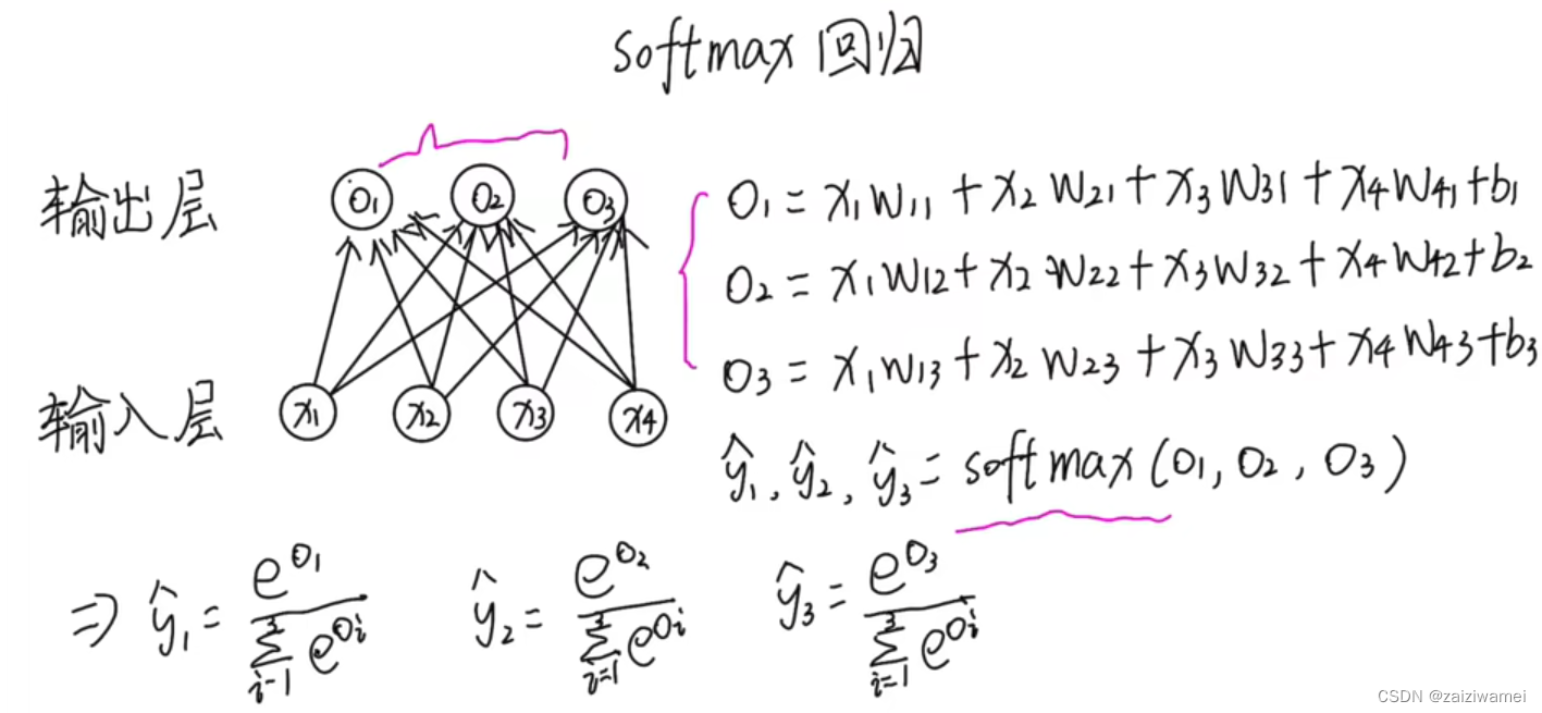
4.8 log_softmax函数

在这里插入图片描述

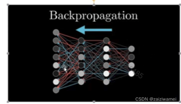
4.9 反向传播

在这里插入图片描述

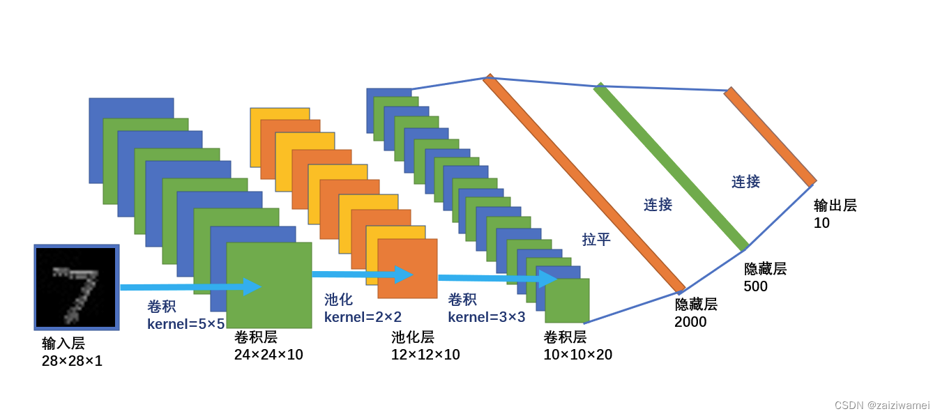
5. 网络结构

在这里插入图片描述

6. 完整的模型训练套路

6.1 加载库

代码如下（示例）：

import torch
import torch.nn as nn
import torch.nn.functional as F
import torch.optim as optim
from torchvision import datasets,transforms
from torch.utils.tensorboard import SummaryWriter  # 加载图像的包
from torch.utils.data import DataLoader
import numpy as np

6.2 定义超参数

代码如下（示例）：

batch_size = 64  # 每批处理的数据
device = torch.device("cuda" if torch.cuda.is_available() else "cpu")  # 是否用GPU进行训练
epochs = 20  # 训练数据集的轮次
train_loss_record = np.zeros(epochs) # 定义训练损失
test_loss_record = np.zeros(epochs) # 定义测试损失
Accuracy_record = np.zeros(epochs) # 定义准确率

6.3 构建pipeline对图像做处理

代码如下（示例）：

# 3 构建pipeline,对图像做处理
pipeline = transforms.Compose([
    transforms.ToTensor(),  # 将图片转换成tensor
    transforms.Normalize((0.1307),(0.3081))  # 正则化,降低模型复杂度
])

6.4 下载、加载数据

代码如下（示例）：

# 下载数据集
train_set = datasets.MNIST("data",train=True, download=True, transform=pipeline)
test_set = datasets.MNIST("data",train=False, download=True, transform=pipeline)

# 加载数据
train_loader = DataLoader(train_set, batch_size=batch_size, shuffle=True)  # shuffle=True,将数据集打乱
test_loader = DataLoader(test_set, batch_size=batch_size, shuffle=True)  # shuffle=True,将数据集打乱

6.5 构建网络模型

代码如下（示例）：

class Digit(nn.Module):
    def __init__(self):
        super(Digit, self).__init__()
        self.conv1 = nn.Conv2d(1, 10, 5)  # 1:灰度图片的通道为1,10：输出通道，5：kernel,
        self.conv2 = nn.Conv2d(10, 20, 3) # 10:输入通道，20：输出通道，3：kernel
        self.linear1 = nn.Linear(20*10*10, 500)  # 全连接层 20*10*10:输入通道，500：输出通道，
        self.linear2 = nn.Linear(500, 10)  # 全连接层 10:输入通道，10：输出通道，
    # 前向传播函数
    def forward(self,x):
        input_size = x.size(0)  # 图像尺寸构成 batch_size*1*28*28,
        x = self.conv1(x)  # 输入：batch*28*28，输出：batch*24*24 计算过程：28-5+1= 24
        x = F.relu(x)  # 激活函数：
        x = F.max_pool2d(x,2,2)  # 池化层：对图片进行压缩，进行下采样的一种方法，有最大池化与平均池化，池化盒核为2*2
                                 # 输入: batch*10*10*24*24 输出：batch*10*10*12
        x = self.conv2(x)  # 输入：batch*10*12*12 输出：batch*20*10*10 (12-3+1=10)
        x = F.relu(x)  # 激活函数：

        x = x.view(input_size,-1)  # 拉平，  -1：自动计算维度
                                   # 输入：batch*20*100*10   输出：2000
        x = self.linear1(x)  # 输入：batch*2000，输出：batch*500

        x = F.relu(x)  # 激活函数：shape保持不变
        x = self.linear2(x)  # 激活函数：shape保持不变
                             # 输入：batch*500，输出：batch*10
        output = F.log_softmax(x,dim=1)  # 计算分类后，每个数字的概率值
        return output

6.6 定义优化器

代码如下（示例）：

model = Digit().to(device)
optimizer = optim.Adam(model.parameters())  # 采用Adam优化器

6.7 定义训练方法

代码如下（示例）：

def train_model(model, device, train_loader, optimizer, epoch):
    #  模型训练
    model.train( )
    for batch_index, (data,target) in enumerate(train_loader):
        # 部署到device上
        data, target = data.to(device),target.to(device)
        # 梯度初始化为0
        optimizer.zero_grad()
        # 训练后的结果
        output = model(data)
        # 计算损失
        loss = F.cross_entropy(output,target)
        # 找到概率值最大的下标
        pred = output.max(1,keepdim=True)  #
        # 反向传播
        loss.backward()
        # 参数优化
        optimizer.step()
        if batch_index % 3000 == 0:
            print("Train Epoch:{}\t Loss:{:.6f}".format(epoch, loss.item()))
            train_loss_record[epoch]=loss.item()优化器

6.8 定义测试方法

代码如下（示例）：

def test_model(model, device, test_loader):
    #  模型验证
    model.eval( )
    # 正确率
    correct = 0.0
    # 测试损失
    test_loss = 0.0
    with torch.no_grad():   # 不计算梯度，也不进行反向传播
        for data, target in test_loader:
            # 部署到device上
            data, target = data.to(device), target.to(device)
            # 测试数据
            output = model(data)
            # 计算测试损失
            test_loss += F.cross_entropy(output,target).item()
            # 找到概率值最大下标
            pred = output.max(1, keepdim=True)[1]  #
            # 累计正确率
            correct += pred.eq(target.view_as(pred)).sum().item()
        test_loss /= len(test_loader.dataset)
        print("Test---Average loss :{:.4f},Accuracy : {:.3f}\n".format(
            test_loss, 100.0 * correct / len(test_loader.dataset)))
        test_loss_record[epoch] = test_loss
        Accuracy_record[epoch] = 100.0 * correct / len(test_loader.dataset)

6.9 模型训练与保存

调用方法7、8进行模型训练，并对测试集模型进行保存
代码如下（示例）：

for epoch in range(0,epochs):
    #训练模型
    train_model(model, device, train_loader,optimizer,epoch)
    test_model(model, device, test_loader)
    # 保存模型
    torch.save(test_model, "D:\\document\\document\\major_study\\Machine-Learning\\实践项目\\model_{}.pth".format(epoch))
    #torch.save(model, "D:\\document\\document\\major_study\\Machine - Learning\\实践项目\\model_{}.pth".format(epoch))
    #D:\document\document\major_study\Machine-Learning\实践项目
    print("模型已保存")

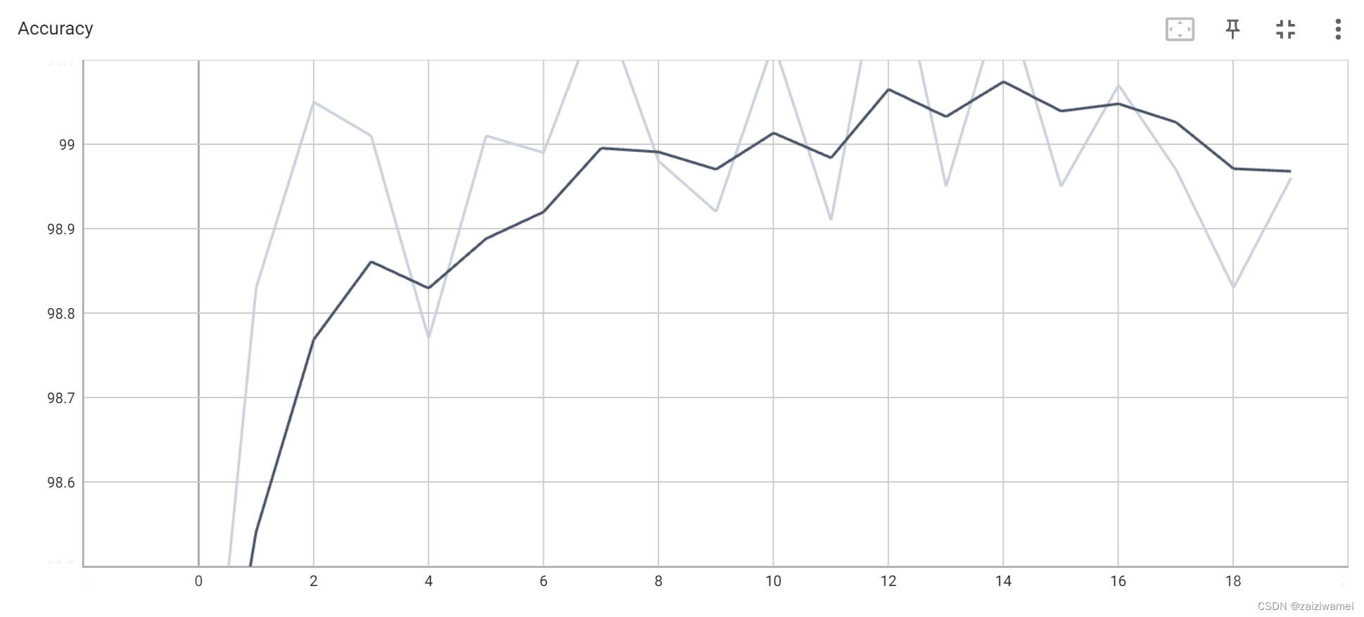
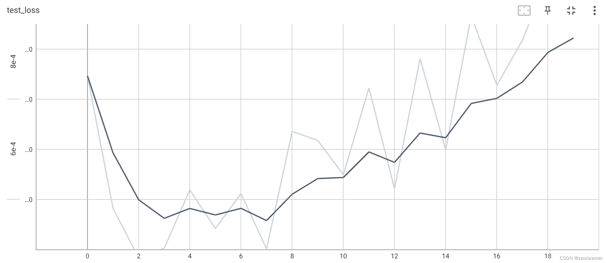
6.10 用TransBoard绘制损失与准确

代码如下（示例）：

writer = SummaryWriter("curve")  # 日志文件名（此处为logs）以及文件位置，默认为当前文件夹
for i in range(epochs):
    writer.add_scalar("train_loss", train_loss_record[i], i)  # 表标题，y轴，x轴
    writer.add_scalar("test_loss", test_loss_record[i], i)  # 表标题，y轴，x轴
    writer.add_scalar("Accuracy", Accuracy_record[i], i)  # 表标题，y轴，x轴
writer.close()

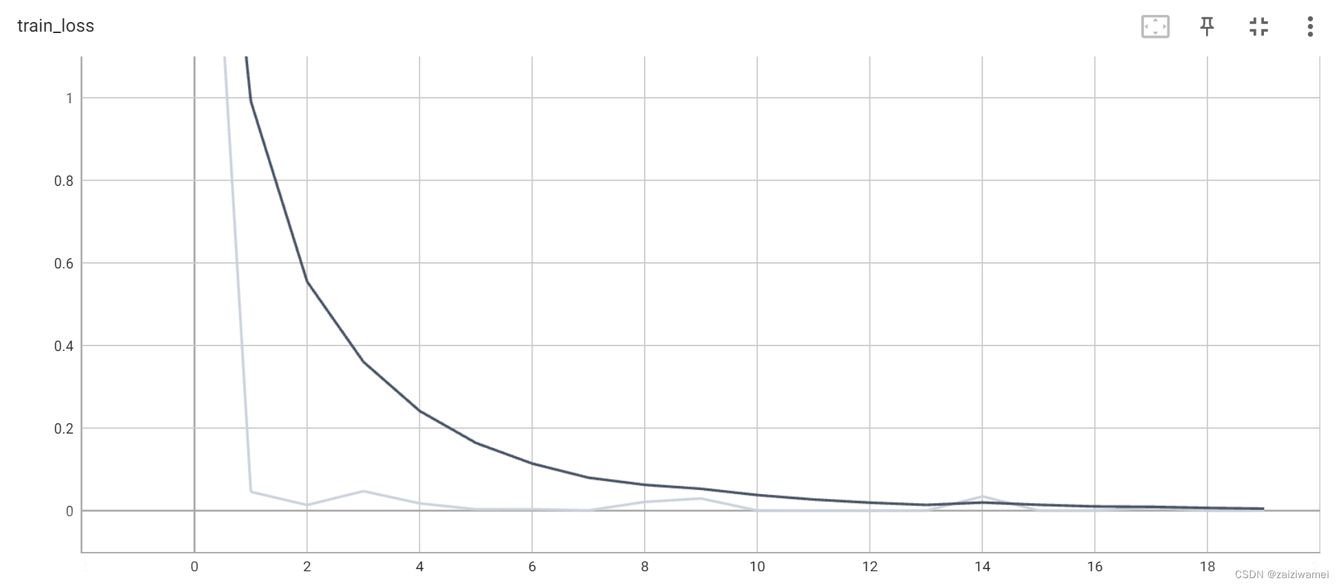
6.11 输出结果

程序输出20个.pth的model文件；
并在TransBoard界面生成相应的图像。
训练损失：
在这里插入图片描述

准确率：
在这里插入图片描述 测试损失：

在这里插入图片描述

7 模型验证

既然我们通过训练获得了手写体模型的特征参数，那我们应该通过输入一张手写体图像来验证其好坏。

在相应文件夹下保存以下图片
在这里插入图片描述
模型验证代码如下：

# 1 加载库
import torch
from PIL import Image
import torchvision
from torch import nn
from torch.nn import Conv2d, MaxPool2d, Flatten, Linear
import torch.nn.functional as F


# 2.1 打开图像
img_path = "D:\\document\\document\\major_study\\Machine-Learning\\实践项目\\digit.jpg"
img = Image.open(img_path)
img = img.convert('RGB')


# 2.2 修改图像格式
transform = torchvision.transforms.Compose([
     torchvision.transforms.Resize((28, 28)),
     torchvision.transforms.ToTensor()
     ])
img = transform(img)
img = torch.reshape(img[0], (1, 28, 28))

# 3 构建网络模型
class Digit(nn.Module):
    def __init__(self):
        super(Digit, self).__init__()
        self.conv1 = nn.Conv2d(1, 10, 5)  # 1:灰度图片的通道为1,10：输出通道，5：kernel,
        self.conv2 = nn.Conv2d(10, 20, 3) # 10:输入通道，20：输出通道，3：kernel
        self.linear1 = nn.Linear(20*10*10, 500)  # 全连接层 20*10*10:输入通道，500：输出通道，
        self.linear2 = nn.Linear(500, 10)  # 全连接层 10:输入通道，10：输出通道，
    # 前向传播函数
    def forward(self,x):
        input_size = x.size(0)  # 图像尺寸构成 batch_size*1*28*28,
        x = self.conv1(x)  # 输入：batch*28*28，输出：batch*24*24 计算过程：28-5+1= 24
        x = F.relu(x)  # 激活函数：
        x = F.max_pool2d(x,2,2)  # 池化层：对图片进行压缩，进行下采样的一种方法，有最大池化与平均池化，池化盒核为2*2
                                 # 输入: batch*10*10*24*24 输出：batch*10*10*12
        x = self.conv2(x)  # 输入：batch*10*12*12 输出：batch*20*10*10 (12-3+1=10)
        x = F.relu(x)  # 激活函数：

        x = x.view(input_size,-1)  # 拉平，  -1：自动计算维度
                                   # 输入：batch*20*100*10   输出：2000
        x = self.linear1(x)  # 输入：batch*2000，输出：batch*500

        x = F.relu(x)  # 激活函数：shape保持不变
        x = self.linear2(x)  # 激活函数：shape保持不变
                             # 输入：batch*500，输出：batch*10
        output = F.log_softmax(x,dim=1)  # 计算分类后，每个数字的概率值
        return output
# 4 加载模型
model = torch.load("D:\\document\\document\\major_study\\Machine-Learning\\实践项目\\model_19.pth")
model.eval()
with torch.no_grad():
     output = model(img.cuda())#注意，用GPU训练的模型必须用GPU加载
print(output.argmax(1))

输出：
tensor([7], device='cuda:0') #对应输入数字7

总结

以上就是今天要讲的内容，本文仅仅简单介绍了机器学习最基础的实例-手写体识别。

华为云开发者联盟

为开发者提供学习成长、分享交流、生态实践、资源工具等服务，帮助开发者快速成长。

更多推荐

通过HPA+CronHPA组合应对业务复杂弹性伸缩场景

华为云开发者联盟

FT-FMEA融合混沌演练，零售运营系统韧性架构在线验证实践

华为云开发者联盟

如何使用Python和Plotly绘制3D图形

华为云开发者联盟

所有评论(0)

查看更多评论

zaiziwamei

@qq_40940944

已为社区贡献1条内容

深度学习实际—手写体识别

zaiziwamei

文章目录

前言

1. 什么是机器识别手写数字？

2. MNIST数据集是什么？

3. 显示MNIST数据集

4. 名词解释

4. 1 图像

4. 2 卷积层

4. 3 池化层

4. 4 线性层

4. 5 激活函数

4. 6 损失函数

4.7 正则化

4.8 log_softmax函数

4.9 反向传播

5. 网络结构

6. 完整的模型训练套路

6.1 加载库

6.2 定义超参数

6.3 构建pipeline对图像做处理

6.4 下载、加载数据

6.5 构建网络模型

6.6 定义优化器

6.7 定义训练方法

6.8 定义测试方法

6.9 模型训练与保存

6.10 用TransBoard绘制损失与准确

6.11 输出结果

7 模型验证

总结

所有评论(0)

zaiziwamei