decision function是sklearn机器学习框架的分类器类（如SVC, Logistic Regression）中的一种method。该method基本上返回一个Numpy数组，其中每个元素表示分类器对x_test的预测样本是位于超平面的右侧还是左侧，以及离超平面有多远。

它还告诉我们，分类器为x_test预测的每个值是正值(大幅度正值)，还是负值(大幅度负值)，以及相应的信任程度。

decision function method背后的数学:

让我们考虑SVM对于线性可分二进制类的分类问题:

损失函数:

这种线性可分的二分类的假设:

优化算法最小化cost function，以找到假设的模型参数的最佳值，从而:

当我们将数据实例传递给决策函数方法时，实际上会发生什么？

该数据样本在该假设中被替换，该假设的模型参数已经通过最小化成本函数找到，并且返回由该假设输出的值，如果实际输出是1，则该值将> 1，或者如果实际输出是0，则该值将<-1。这个返回值确实代表了超平面的哪一侧，以及给定的数据样本离它有多远。

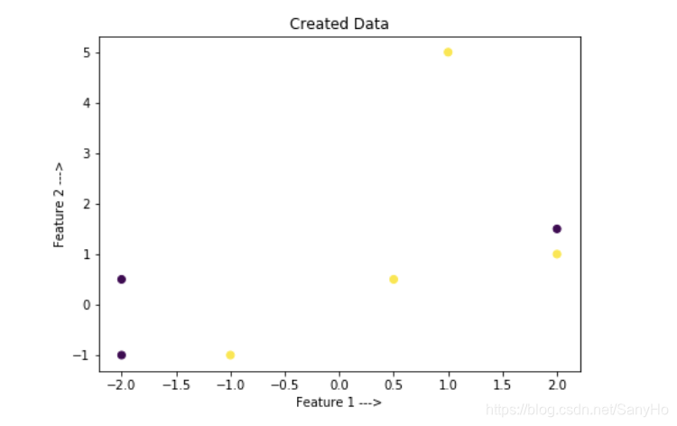
Code: 创建我们自己的数据集并绘制输入

# This code may not run on GFG IDE
# As required modules are not available.

# Create a simple data set
# Binary-Class Classification.

# Import Required Modules.
import matplotlib.pyplot as plt
import numpy as np

# Input Feature X.
x = np.array([[2, 1.5], [-2, -1], [-1, -1], [2, 1],
			[1, 5], [0.5, 0.5], [-2, 0.5]])

# Input Feature Y.
y = np.array([0, 0, 1, 1, 1, 1, 0])

# Training set Featute x_train.
x_train = np.array([[2, 1.5], [-2, -1], [-1, -1], [2, 1]])

# Training set Target Variable y_train.
y_train = np.array([0, 0, 1, 1])

# Test set Featute x_test.
x_test = np.array([[1, 5], [0.5, 0.5], [-2, 0.5]])

# Test set Target Variable y_test
y_test = np.array([1, 1, 0])

# Plot the obtained data
plt.scatter(x[:, 0], x[:, 1], c = y)
plt.xlabel('Feature 1 --->')
plt.ylabel('Feature 2 --->')
plt.title('Created Data')

Code: 训练模型

# This code may not run on GFG IDE
# As required modules are not available.

# Import SVM Class from sklearn.
from sklearn.svm import SVC
clf = SVC()

# Train the model on the training set.
clf.fit(x_train, y_train)

# Predict on Test set
predict = clf.predict(x_test)
print('Predicted Values from Classifier:', predict)
print('Actual Output is:', y_test)
print('Accuracy of the model is:', clf.score(x_test, y_test))

Predicted Values from Classifier: [0 1 0]
Actual Output is: [1 1 0]
Accuracy of the model is: 0.6666666666666666

# This code may not run on GFG IDE
# As required modules are not available.

# Using Decision Function Method Present in svc class
Decision_Function = clf.decision_function(x_test)
print('Output of Decision Function is:', Decision_Function)
print('Prediction for x_test from classifier is:', predict)

Output of Decision Function is: [-0.04274893  0.29143233 -0.13001369]
Prediction for x_test from classifier is: [0 1 0]

从上面的输出中，我们可以得出结论，决策函数输出表示分类器对x_test的预测样本是位于超平面的右侧还是左侧，以及离它有多远。它还告诉我们分类器为x_test预测的每个值是正的(大幅度正值)还是负的(大幅度负值)。

# This code may not run on GFG IDE
# As required modules are not available.

# To Plot the Decision Boundary.
arr1 = np.arange(x[:, 0].min()-1, x[:, 0].max()+1, 0.01)
arr2 = np.arange(x[:, 1].min()-1, x[:, 1].max()+1, 0.01)

xx, yy = np.meshgrid(arr1, arr2)
input_array = np.array([xx.ravel(), yy.ravel()]).T
labels = clf.predict(input_array)

plt.figure(figsize =(10, 7))
plt.contourf(xx, yy, labels.reshape(xx.shape), alpha = 0.1)
plt.scatter(x_test[:, 0], x_test[:, 1], c = y_test.ravel(), alpha = 1)
plt.xlabel('Feature 1')
plt.ylabel('Feature 2')
plt.title('Decision Boundary')

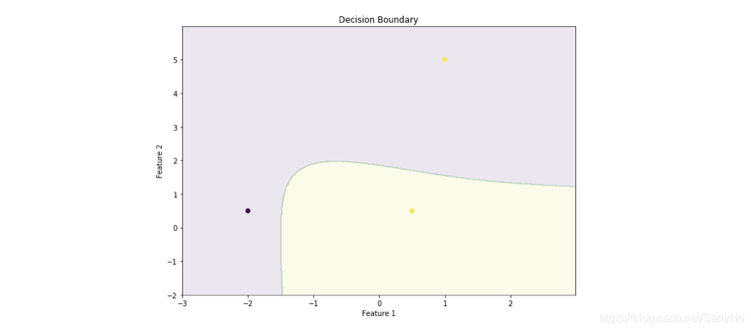
决策函数输出的优点是为x_test设置决策阈值和预测新的输出，这样如果我们的项目分别面向精度或面向召回，我们就可以获得期望的精度或召回值。

*翻译自ML – Decision Function