如果目标函数或约束条件中包含非线性函数，就称这种规划问题为非线性规划问题。一般来说，求解非线性规划要比线性规划困难得多，而且，不像线性规划有通用的方法。非线性规划目前还没有适用于各种问题的一般算法，各个方法都有自己特定的适用范围。

一般形式

非线性规划的一般形式为
$$\begin{array}{c}\min f(x),\\ \text{ s.t. }\{\begin{array}{l}G(x)\le 0,\\ H(x)=0,\end{array}\end{array}$$

其中 $G(x)={\left[g_1(x),g_2(x),\cdots ,g_m(x)\right]}^T$, $H(x)={\left[h_1(x),h_2(x),\cdots ,h_l(x)\right]}^T$，$f,g_i,h_j$ 都是定义在 ${\mathbb{R}}^n$ 上的实值函数

Python 求解

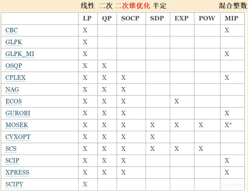
在使用 Python 求解非线性规划时要注意求解器的适用范围，各求解器的适用范围如下

1. scipy.optimize.minimize 函数

调用方式:

import scipy
res = scipy.optimize.minimize(fun, x0, args=(), method=None, jac=None, hess=None, hessp=None, bounds=None, constraints=(), tol=None, callback=None, options=None)

参数:

fun: 目标函数: fun(x, *args) x 是形状为 (n,) 的一维数组 (n 是自变量的数量)

x0: 初值, 形状 (n，) 的 ndarray

method: 求解器的类型，如果未给出，有约束时则选择 'SLSQP'。

constraints: 求解器 SLSQP 的约束被定义为字典的列表，字典用到的字段主要有：

• 'type': str: 约束类型：“eq” 表示等式，“ineq” 表示不等式 (SLSQP 的不等式约束是 $f(x)\ge 0$ 的形式)
• 'fun': 可调用的函数或匿名函数：定义约束的函数

bounds: 变量界限

返回:

print(res.fun) #最优值
print(res.success) #求解状态
print(res.x)  #最优解

e.g.

from scipy.optimize import minimize
import numpy as np
def obj(x):
    # 定义目标函数
    return f(x)
LB=[LB]; UB=[UB] # n 个元素的列表
cons=[{'type':'ineq','fun':lambda x: G(x)},{'type':'eq','fun':lambda x: H(x)}]
bd=tuple(zip(LB, UB)) # 生成决策向量界限的元组
res=minimize(obj,np.ones(n),constraints=cons,bounds=bd) #第2个参数为初值
print(res.fun) #最优值
print(res.success) #求解状态
print(res.x)  #最优解

例 1

$$\min \frac{2+x_1}{1+x_2}-3x_1+4x_3\text{, }$$

$$s.t.0.1\le x_i\le 0.9,i=1,2,3$$

from scipy.optimize import minimize
from numpy import ones
def obj(x):
    x1,x2,x3=x
    return (2+x1)/(1+x2)-3*x1+4*x3
LB=[0.1]*3; UB=[0.9]*3
bound=tuple(zip(LB, UB))   
res=minimize(obj,ones(3),bounds=bound) 
print(res.fun,'\n',res.success,'\n',res.x)  #输出最优值、求解状态、最优解

-0.7736842105263159 
 True 
 [0.9 0.9 0.1]

例 2

$$\begin{array}{c}\max z=x_1^2+x_2^2+3x_3^2+4x_4^2+2x_5^2-8x_1-2x_2-3x_3-x_4-2x_5,\\ \text{ s.t. }\{\begin{array}{l}{x}_1+x_2+x_3+x_4+x_5\le 400,\\ x_1+2x_2+2x_3+x_4+6x_5\le 800\\ 2x_1+x_2+6x_3\le 200\\ x_3+x_4+5x_5\le 200\\ 0\le x_i\le 99,i=1,2,\cdots ,5.\end{array}\end{array}$$

from scipy.optimize import minimize
import numpy as np
c1=np.array([1,1,3,4,2]); c2=np.array([-8,-2,-3,-1,-2])
A=np.array([[1,1,1,1,1],[1,2,2,1,6],
            [2,1,6,0,0],[0,0,1,1,5]])
b=np.array([400,800,200,200])
obj=lambda x: np.dot(-c1,x**2)+np.dot(-c2,x)
# np.dot()向量点乘或矩阵乘法
cons={'type':'ineq','fun':lambda x:b-A@x}
bd=[(0,99) for i in range(A.shape[1])]
#res=minimize(obj,np.ones(5)*90,constraints=cons,bounds=bd)
res=minimize(obj,np.ones(5),constraints=cons,bounds=bd)
print(res.fun) 
print(res.success) 
print(res.x)

-42677.56889347886
True
[0.00000000e+00 1.43988405e-12 3.33333334e+01 9.90000000e+01
 1.35333333e+01]

本题只能求得局部最优解，可使用不同初值尝试求解

2. cvxopt.solvers 模块求解二次规划

标准型：

$$\begin{array}{c}\min \frac{1}{2}{x}^{T}Px+q^{T}x,\\ \text{ s.t. }\{\begin{array}{l}Ax\le b,\\ Aeq\cdot x=beq.\end{array}\end{array}$$

调用方式:

import numpy as np
from cvxopt import matrix,solvers
sol=solvers.qp(P,q,A,b,Aeq,beq) #二次规划
'''
输入到cvxopt.solvers的矩阵 P,q,A,b,Aeq,beq 都是 cvxopt.matrix 形式
在程序中虽然没有直接使用 NumPy 库中的函数，也要加载
数据如果全部为整型数据，也必须写成浮点型数据
cvxopt.matrix(array,dims) 把array按照dims重新排成矩阵
    省略dims: 如果array为np.array, 则为其原本形式; 
        如果array为list, 则认为 list 中用逗号分隔开的为一"列"
'''
print(sol['x']) #最优解
print(sol['primal objective']) #最优值

例 3

$$\begin{array}{c}\min z=1.5x_1^2+x_2^2+0.85x_3^2+3x_1-8.2x_2-1.95x_3,\\ \text{ s.t. }\{\begin{array}{l}{x}_1+x_3\le 2\\ -x_1+2x_2\le 2\\ x_2+2x_3\le 3\\ x_1+x_2+x_3=3\end{array}\end{array}$$

解:

$$\begin{array}{c}P=\left[\begin{array}{ccc}3& 0& 0\\ 0& 2& 0\\ 0& 0& 1.7\end{array}\right],q=\left[\begin{array}{c}3\\ -8.2\\ -1.95\end{array}\right],A=\left[\begin{array}{ccc}1& 0& 1\\ -1& 2& 0\\ 0& 1& 2\end{array}\right],b=\left[\begin{array}{l}2\\ 2\\ 3\end{array}\right],\end{array}$$

$Aeq=[1,1,1],beq=[3].$

import numpy as np
from cvxopt import matrix,solvers
n=3; P=matrix(0.,(n,n)); #零矩阵
P[::n+1]=[3,2,1.7]; #对角元变为3, 2, 1.7
q=matrix([3,-8.2,-1.95])
A=matrix([[1.,0,1],[-1,2,0],[0,1,2]]).T
b=matrix([2.,2,3])
Aeq=matrix(1.,(1,n)); beq=matrix(3.)
s=solvers.qp(P,q,A,b,Aeq,beq)
print("最优解为：",s['x'])
print("最优值为：",s['primal objective'])

     pcost       dcost       gap    pres   dres
 0: -1.3148e+01 -4.4315e+00  1e+01  1e+00  9e-01
 1: -6.4674e+00 -7.5675e+00  1e+00  2e-16  1e-16
 2: -7.1538e+00 -7.1854e+00  3e-02  1e-16  4e-16
 3: -7.1758e+00 -7.1761e+00  3e-04  1e-16  2e-15
 4: -7.1760e+00 -7.1760e+00  3e-06  5e-17  2e-15
Optimal solution found.
最优解为： [ 8.00e-01]
[ 1.40e+00]
[ 8.00e-01]

最优值为： -7.1759977687772745

3. cvxpy 库

使用方式与这里相似，只需选择支持的求解器即可

例 4

$$\begin{array}{c}\min z=x_1^2+x_2^2+3x_3^2+4x_4^2+2x_5^2-8x_1-2x_2-3x_3-x_4-2x_5,\\ \text{ s.t. }\{\begin{array}{l}0\le x_i\le 99,\text{ 且 }{x}_i\text{ 为整数 }(i=1,\cdots ,5),\\ x_1+x_2+x_3+x_4+x_5\le 400,\\ x_1+2x_2+2x_3+x_4+6x_5\le 800\\ 2x_1+x_2+6x_3\le 200\\ x_3+x_4+5x_5\le 200.\end{array}\end{array}$$

import cvxpy as cp
import numpy as np
c1=np.array([1, 1, 3, 4, 2])
c2=np.array([-8, -2, -3, -1, -2])
a=np.array([[1, 1, 1, 1, 1], [1, 2, 2, 1, 6], [2, 1, 6, 0, 0], [0, 0, 1, 1, 5]])
b=np.array([400, 800, 200, 200])
x=cp.Variable(5,integer=True)
obj=cp.Minimize(c1@(x**2)+c2@x)
con=[0<=x, x<=99, a@x<=b]
prob = cp.Problem(obj, con)
prob.solve()
print("最优值为:",prob.value)
print("最优解为:",x.value)

最优值为: -17.0
最优解为: [4. 1. 0. 0. 0.]