Python二手车价格预测（二）—— 模型训练及可视化

Python二手车价格预测之模型训练与可视化，使用7种经典回归模型进行训练，并对结果进行可视化。

_HXZ

10726人浏览 · 2022-04-13 11:14:03

_HXZ · 2022-04-13 11:14:03 发布

系列文章目录

一、Python数据分析-二手车数据获取用于机器学习二手车价格预测

二、Python二手车价格预测（一）—— 数据处理

文章目录

系列文章目录
前言
一、明确任务
二、模型训练
三、重要特征筛选
结语

前言

前面分享了二手车数据获取的内容，又对获取的原始数据进行了数据处理，相关博文可以访问上面链接。许多朋友私信我问会不会出模型，今天模型baseline来了！允许我抛砖引玉，有什么地方描述的不恰当或者有问题，请各位朋友们评论指正！

一、明确任务

一般的预测任务分为回归任务和分类任务，二手车的价格是一个连续值，因此二手车价格预测是一个回归任务。
回归任务的模型有很多，如：线性回归、K近邻（KNN）、岭回归、多层感知机、决策树回归、极限树回归、随机森林、梯度提升树……
诸多模型中有一部分模型是通过多个弱学习器集成起来的模型，像随机森林、Voting等，它们具有更强的学习能力，集成多个单一学习器得到最终结果，一般集成模型的预测效果表现都很良好。
为了给大家提供一个二手车价格预测的baseline，我将选取几个经典模型进行训练。

二、模型训练

1.引入库

代码如下：

# 写在前面，大家可以关注一下微信公众号：吉吉的机器学习乐园
# 可以通过后台获取数据，不定期分享Python，Java、机器学习等相关内容

import pandas as pd
import numpy as np
import matplotlib.pyplot as plt
from matplotlib.pyplot import MultipleLocator
import sys
import seaborn as sns
import warnings
warnings.filterwarnings("ignore")
plt.rcParams['font.sans-serif'] = ['SimHei']  # 用来正常显示中文标签
plt.rcParams['axes.unicode_minus'] = False  # 用来正常显示负号
pd.set_option('display.max_rows', 100,'display.max_columns', 1000,"display.max_colwidth",1000,'display.width',1000)

from sklearn.metrics import *
from sklearn.linear_model import *
from sklearn.neighbors import *
from sklearn.svm import *
from sklearn.neural_network import *
from sklearn.tree import *
from sklearn.ensemble import *
from xgboost import *
import lightgbm as lgb
import tensorflow as tf
from tensorflow.keras import layers
from sklearn.preprocessing import *
from sklearn.ensemble import RandomForestRegressor as RFR
from sklearn.model_selection import *

2.读入数据

代码如下：

# final_data.xlsx 是上一次分享最后数据处理后的
data = pd.read_excel("final_data.xlsx", na_values=np.nan

# 将数据划分输入和结果集
X = data[ data.columns[1:] ]
y_reg = data[ data.columns[0] ]

# 切分训练集和测试集， random_state是切分数据集的随机种子，要想复现本文的结果，随机种子应该一致
x_train, x_test, y_train, y_test = train_test_split(X, y_reg, test_size=0.3, random_state=42)

3.评价指标

平均绝对误差（MAE）

平均绝对误差的英文全称为 Mean Absolute Error，也称之为 L1 范数损失。是通过计算预测值和真实值之间的距离的绝对值的均值，来衡量预测值与真实值之间的距离。计算公式如下：

MAE

均方误差（MSE）

均方误差英文全称为 Mean Squared Error，也称之为 L2 范数损失。通过计算真实值与预测值的差值的平方和的均值来衡量距离。计算公式如下：

MSE

均方根误差（RMSE）

均方根误差的英文全称为 Root Mean Squared Error，代表的是预测值与真实值差值的样本标准差。计算公式如下：

RMSE

决定系数（R2）

决定系数评估的是预测模型相对于基准模型（真实值的平均值作为预测值）的好坏程度。计算公式如下：

最好的模型预测的 R2 的值为 1，表示预测值与真实值之间是没有偏差的；
但是最差的模型，得到的 R2 的值并不是 0，而是会得到负值；
当模型的 R2 值为负值，表示模型预测结果比基准模型（均值模型）表现要差；
当模型的 R2 值大于 0，表示模型的预测结果比使用均值预测得到的结果要好。

定义评价指标函数：

# 评价指标函数定义，其中R2的指标可以由模型自身得出，后面的score即为R2
def evaluation(model):
    ypred = model.predict(x_test)
    mae = mean_absolute_error(y_test, ypred)
    mse = mean_squared_error(y_test, ypred)
    rmse = sqrt(mse)
    print("MAE: %.2f" % mae)
    print("MSE: %.2f" % mse)
    print("RMSE: %.2f" % rmse)
    return ypred

4.线性回归

代码如下：

model_LR = LinearRegression()
model_LR.fit(x_train, y_train)
print("params: ", model_LR.get_params())
print("train score: ", model_LR.score(x_train, y_train))
print("test score: ", model_LR.score(x_test, y_test))
predict_y = evaluation(model_LR)

输出结果：

params:  {'copy_X': True, 'fit_intercept': True, 'n_jobs': None, 'normalize': False}
train score:  0.823587700962806
test score:  0.7654427047191524
MAE: 1.97
MSE: 25.90
RMSE: 5.09

我们可以将 y_test 转换为 numpy 的 array 形式，方便后面的绘图。

test_y = np.array(y_test)

由于数据量较多，我们取预测结果和真实结果的前50个数据进行绘图。

plt.figure(figsize=(10,10))
plt.title('线性回归-真实值预测值对比')
plt.plot(predict_y[:50], 'ro-', label='预测值')
plt.plot(test_y[:50], 'go-', label='真实值')
plt.legend()
plt.show()

线性回归
上图中，绿色点为真实值，红色点为预测值，当两点几乎重合时，说明模型的预测结果十分接近。

5.K近邻

代码如下：

model_knn = KNeighborsRegressor()
model_knn.fit(x_train, y_train)
print("params: ", model_knn.get_params())
print("train score: ", model_knn.score(x_train, y_train))
print("test score: ", model_knn.score(x_test, y_test))
predict_y = evaluation(model_knn)

输出结果：

params:  {'algorithm': 'auto', 'leaf_size': 30, 'metric': 'minkowski', 'metric_params': None, 'n_jobs': None, 'n_neighbors': 5, 'p': 2, 'weights': 'uniform'}
train score:  0.8701966571367806
test score:  0.7886892618747352
MAE: 1.35
MSE: 23.33
RMSE: 4.83

绘图：

plt.figure(figsize=(10,10))
plt.title('KNN-真实值预测值对比')
plt.plot(predict_y[:50], 'ro-', label='预测值')
plt.plot(test_y[:50], 'go-', label='真实值')
plt.legend()
plt.show()

KNN

6.决策树回归

代码如下：

model_dtr = DecisionTreeRegressor(max_depth = 5, random_state=30)
model_dtr.fit(x_train, y_train)
print("params: ", model_dtr.get_params())
print("train score: ", model_dtr.score(x_train, y_train))
print("test score: ", model_dtr.score(x_test, y_test))
predict_y = evaluation(model_dtr)

在这里，决策树学习器加入了一个 max_depth 的参数，这个参数限定了树的最大深度，设置这个参数的主要原因是为了防止模型过拟合

输出结果：

params:  {'criterion': 'mse', 'max_depth': 5, 'max_features': None, 'max_leaf_nodes': None, 'min_impurity_decrease': 0.0, 'min_impurity_split': None, 'min_samples_leaf': 1, 'min_samples_split': 2, 'min_weight_fraction_leaf': 0.0, 'presort': False, 'random_state': 30, 'splitter': 'best'}
train score:  0.8339532311129941
test score:  0.7857733129009127
MAE: 2.16
MSE: 18.37
RMSE: 4.29

如果不限定树的最大深度会发生什么呢？

model_dtr = DecisionTreeRegressor(random_state=30)
model_dtr.fit(x_train, y_train)
print("params: ", model_dtr.get_params())
print("train score: ", model_dtr.score(x_train, y_train))
print("test score: ", model_dtr.score(x_test, y_test))
predict_y = evaluation(model_dtr)

输出结果：

params:  {'criterion': 'mse', 'max_depth': None, 'max_features': None, 'max_leaf_nodes': None, 'min_impurity_decrease': 0.0, 'min_impurity_split': None, 'min_samples_leaf': 1, 'min_samples_split': 2, 'min_weight_fraction_leaf': 0.0, 'presort': False, 'random_state': 30, 'splitter': 'best'}
train score:  0.999999225529954
test score:  0.8673942873037808
MAE: 1.16
MSE: 14.64
RMSE: 3.83

获得树的最大深度：

model_dtr.get_depth()

输出结果：

我们发现，在不限定树的最大深度时，决策树模型的训练得分（R2）为：0.999999225529954，但测试得分仅为：0.8673942873037808。
这就是模型过拟合，在训练数据上的表现非常良好，当用未训练过的测试数据进行预测时，模型的泛化能力不足，导致测试结果不理想。
感兴趣的同学可以自行查阅关于决策树剪枝的过程。

绘图：

plt.figure(figsize=(10,10))
plt.title('决策树回归-真实值预测值对比')
plt.plot(predict_y[:50], 'ro-', label='预测值')
plt.plot(test_y[:50], 'go-', label='真实值')
plt.legend()
plt.show()

决策树回归

7.随机森林

代码如下：

model_rfr = RandomForestRegressor(random_state=30)
model_rfr.fit(x_train, y_train)
print("params: ", model_rfr.get_params())
print("train score: ", model_rfr.score(x_train, y_train))
print("test score: ", model_rfr.score(x_test, y_test))
predict_y = evaluation(model_rfr)

输出结果：

params:  {'bootstrap': True, 'criterion': 'mse', 'max_depth': None, 'max_features': 'auto', 'max_leaf_nodes': None, 'min_impurity_decrease': 0.0, 'min_impurity_split': None, 'min_samples_leaf': 1, 'min_samples_split': 2, 'min_weight_fraction_leaf': 0.0, 'n_estimators': 10, 'n_jobs': None, 'oob_score': False, 'random_state': 30, 'verbose': 0, 'warm_start': False}
train score:  0.9873589573962257
test score:  0.9004628017201377
MAE: 0.88
MSE: 10.99
RMSE: 3.32

绘图：

plt.figure(figsize=(10,10))
plt.title('随机森林-真实值预测值对比')
plt.plot(predict_y[:50], 'ro-', label='预测值')
plt.plot(test_y[:50], 'go-', label='真实值')
plt.legend()
plt.show()

随机森林

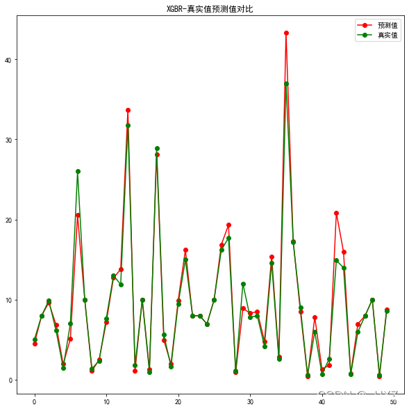
8.XGBoost

XGboost是华盛顿大学博士陈天奇创造的一个梯度提升（Gradient Boosting）的开源框架。至今可以算是各种数据比赛中的大杀器，被大家广泛地运用。

代码如下：

model_xgbr = XGBRegressor(n_estimators = 200, max_depth=5, random_state=1024)
model_xgbr.fit(x_train, y_train)
print("params: ", model_xgbr.get_params())
print("train score: ", model_xgbr.score(x_train, y_train))
print("test score: ", model_xgbr.score(x_test, y_test))
predict_y = evaluation(model_xgbr)

输出结果：

params:  {'objective': 'reg:squarederror', 'base_score': 0.5, 'booster': 'gbtree', 'colsample_bylevel': 1, 'colsample_bynode': 1, 'colsample_bytree': 1, 'gamma': 0, 'gpu_id': -1, 'importance_type': 'gain', 'interaction_constraints': '', 'learning_rate': 0.300000012, 'max_delta_step': 0, 'max_depth': 5, 'min_child_weight': 1, 'missing': nan, 'monotone_constraints': '()', 'n_estimators': 200, 'n_jobs': 0, 'num_parallel_tree': 1, 'random_state': 1024, 'reg_alpha': 0, 'reg_lambda': 1, 'scale_pos_weight': 1, 'subsample': 1, 'tree_method': 'exact', 'validate_parameters': 1, 'verbosity': None}
train score:  0.9897272945187993
test score:  0.8923618501911923
MAE: 0.88
MSE: 11.88
RMSE: 3.45

绘图：

plt.figure(figsize=(10,10))
plt.title('XGBR-真实值预测值对比')
plt.plot(predict_y[:50], 'ro-', label='预测值')
plt.plot(test_y[:50], 'go-', label='真实值')
plt.legend()
plt.show()

XGBR

9.集成模型Voting

Voting可以简单理解为将各个模型的结果加权平均，也是使用较多的一种集成模型。

代码如下：

model_voting = VotingRegressor(estimators=[('model_LR', model_LR),
                                           ('model_knn', model_knn), 
                                           ('model_dtr', model_dtr),
                                           ('model_rfr', model_rfr),
                                           ('model_xgbr', model_xgbr)])
model_voting.fit(x_train, y_train)
# print("params: ", model_voting.get_params())
print("train score: ", model_voting.score(x_train, y_train))
print("test score: ", model_voting.score(x_test, y_test))
predict_y = evaluation(model_voting)

输出结果：

train score:  0.9572901767964346
test score:  0.8964163648799375
MAE: 1.08
MSE: 11.44
RMSE: 3.38

绘图：

plt.figure(figsize=(10,10))
plt.title('集成模型voting-真实值预测值对比')
plt.plot(predict_y[:50], 'ro-', label='预测值')
plt.plot(test_y[:50], 'go-', label='真实值')
plt.legend()
plt.show()

Voting

10.Tensorflow神经网络

使用Tensorflow前需要安装，本文使用的是tensorflow2.0.0版本。

为了使模型快速收敛，首先需要将数据标准化。

代码如下：

scaler = StandardScaler()
x_train_scaled = scaler.fit_transform(x_train)
x_test_scaled = scaler.transform(x_test)

train_x = np.array(x_train_scaled)
test_x = np.array(x_test_scaled)
train_y = np.array(y_train)
test_y = np.array(y_test)


# 1、模型初始化
model_tf = tf.keras.Sequential()

# 2、添加隐藏层，并设置激活函数，这里我们用relu
model_tf.add(layers.Dense(128, activation='relu'))
model_tf.add(layers.Dense(64, activation='relu'))
model_tf.add(layers.Dense(8, activation='relu'))
model_tf.add(layers.Dense(4, activation='relu'))
model_tf.add(layers.Dense(1, activation='relu'))

# 3、初始化输入的shape，189为输入的189维特征
model_tf.build(input_shape =(None,189))

# 4、编译模型
model_tf.compile(optimizer=tf.keras.optimizers.RMSprop(0.001),
             loss=tf.keras.losses.mean_squared_error,
             metrics=['mse', 'mae'])

# 5、模型训练
history = model_tf.fit(train_x, train_y, epochs=200, batch_size=128,
                    validation_split = 0.2, #从测试集中划分80%给训练集
                    validation_freq = 1) #测试的间隔次数为1

# 获取模型训练过程
model_tf.summary()

输出结果：
Tensorflow神经网络
模型训练损失情况：

history_dict = history.history
loss_values = history_dict['loss']
mae=history_dict["mae"]
mse=history_dict["mse"]
val_loss = history_dict['val_loss']
val_mae = history_dict['val_mae']
val_mse = history_dict['val_mse']
epochs = range(1, len(loss_values) + 1)

plt.figure(figsize=(8,5))
plt.plot(range(1, len(loss_values) + 1), loss_values, label = 'Training loss')
plt.plot(range(1, len(val_loss) + 1), val_loss, label = 'Validation loss')
plt.title('Training and validation loss')
plt.xlabel('Epochs')
plt.ylabel('Loss')
plt.legend()
plt.show()

loss

模型MAE：

plt.figure(figsize=(8,5))
plt.plot(range(1, len(mae) + 1), mae, label = 'mae')
plt.plot(range(1, len(val_mae) + 1), val_mae, label = 'val_mae')
plt.title('mean_absolute_error')
plt.xlabel('Epochs')
plt.ylabel('error')
plt.legend()
plt.show()

MAE
模型MSE：

plt.figure(figsize=(8,5))
plt.plot(range(1, len(mse) + 1), mse, label = 'mse')
plt.plot(range(1, len(val_mse) + 1), val_mse, label = 'val_mse')
plt.title('mean_squre_error')
plt.xlabel('Epochs')
plt.ylabel('error')
plt.legend()
plt.show()

MSE
模型评估：

ypred = model_tf.predict(test_x)
mae = mean_absolute_error(test_y, ypred)
mse = mean_squared_error(test_y, ypred)
rmse = sqrt(mse)
print("MAE: %.2f" % mae)
print("MSE: %.2f" % mse)
print("RMSE: %.2f" % rmse)

输出结果：

MAE: 0.94
MSE: 24.03
RMSE: 4.90

11.各模型结果

模型名称	MAE	MSE	RMSE	Train R2	Test R2
线性回归	1.97	25.9	5.09	0.82	0.76
KNN	1.35	23.3	4.83	0.87	0.78
决策树	2.09	23.9	4.89	0.84	0.78
随机森林	0.88	10.99	3.32	0.98	0.90
XGBoost	0.88	11.88	3.45	0.98	0.89
Voting	1.08	11.44	3.38	0.95	0.89
神经网络	0.94	24.0	4.90	0.98	0.78

从上表可以看出，随机森林模型的整体表现最好。当然，这不代表最优结果，因为上述7种模型都没有进行调参优化，经过调参后的各个模型效果还有可能提升。

三、重要特征筛选

为了提升模型效果也可以对数据做特征筛选，这里可以通过相关系数分析法，将影响二手车售价的特征与售价做相关系数计算，pandas包很方便的集成了算法，并且可以通过seaborn、matplotlib等绘图包将相关系数用热力图的方式可视化。

# 这里的列取final_data中，除0-1和独热编码形式的数据
corr_cols = list(data.columns[:28]) + list(data.columns[43:49])
test_data = data[corr_cols]
test_data_corr = test_data.corr()
price_corr = dict(test_data_corr.iloc[0])
price_corr = sorted(price_corr.items(), key=lambda x: abs(x[1]), reverse=True)
# 输出按绝对值排序后的相关系数
print(price_corr)

输出结果，除"售价"外，共有33个特征：

[('售价', 1.0),
 ('新车售价', 0.7839935301900343),
 ('最大功率(kW)', 0.7117612690884588),
 ('最大马力(Ps)', 0.7110554212212731),
 ('最大扭矩(N·m)', 0.696952631401139),
 ('最高车速(km/h)', 0.5419965777866631),
 ('排量(mL)', 0.5330405118740592),
 ('排量(L)', 0.5308107362792799),
 ('整备质量(kg)', 0.49194473580917225),
 ('官方0-100km/h加速(s)', -0.48176542342318535),
 ('宽度(mm)', 0.4714397275896106),
 ('轴距(mm)', 0.46166756230018036),
 ('气缸数(个)', 0.4454272911508132),
 ('油箱容积(L)', 0.437777686409757),
 ('后轮距(mm)', 0.38050056092464896),
 ('长度(mm)', 0.3713764530321577),
 ('前轮距(mm)', 0.3620381932871346),
 ('最大扭矩转速(rpm)', -0.3350318499883131),
 ('注册日期差（天）', -0.2737947095245184),
 ('出厂日期差（天）', -0.2598892184068559),
 ('工信部综合油耗(L/100km)', 0.21117598576704852),
 ('行驶里程', -0.15837809707633024),
 ('最大功率转速(rpm)', -0.14929627599693607),
 ('行李厢容积(L)', 0.1303796302281349),
 ('每缸气门数(个)', 0.08610716158708019),
 ('压缩比', 0.0820485577972737),
 ('车门数', -0.05405277879497536),
 ('高度(mm)', 0.04866102899154555),
 ('商业险过期日期差（天）', -0.047366786391213236),
 ('交强险过期日期差（天）', -0.04465347803879652),
 ('车船税过期日期差（天）', -0.03694367077131783),
 ('载客/人', -0.03234487106605593),
 ('最小离地间隙(mm)', 0.027822359248097703),
 ('座位数', 0.016036623933084658)]

绘制热力图：

price_corr_cols = [ r[0] for r in price_corr ]
price_data = test_data_corr[price_corr_cols].loc[price_corr_cols]
plt.figure(figsize=(15, 10))
plt.title("相关系数热力图")
ax = sns.heatmap(price_data, linewidths=0.5, cmap='OrRd', cbar=True)
plt.show()

热力图
为了验证相关系数分析出来的重要特征是否对模型有效，我们将模型效果最好的随机森林模型的前33个重要特征输出。

feature_important = sorted(
    zip(x_train.columns, map(lambda x:round(x,4), model_rfr.feature_importances_)),
    key=lambda x: x[1],reverse=True)

for i in range(33):
    print(feature_important[i])

输出结果：

('新车售价', 0.5435)
('最大马力(Ps)', 0.0928)
('注册日期差（天）', 0.077)
('最大扭矩(N·m)', 0.0547)
('最大功率(kW)', 0.05)
('行驶里程', 0.0406)
('出厂日期差（天）', 0.0187)
('高度(mm)', 0.0128)
('驻车制动类型_手刹', 0.0107)
('最大功率转速(rpm)', 0.0098)
('宽度(mm)', 0.007)
('轴距(mm)', 0.0059)
('工信部综合油耗(L/100km)', 0.0052)
('最大扭矩转速(rpm)', 0.0043)
('长度(mm)', 0.0042)
('助力类型_电动助力', 0.0041)
('后轮距(mm)', 0.0038)
('整备质量(kg)', 0.0038)
('挡位个数_5', 0.0035)
('行李厢容积(L)', 0.0027)
('最高车速(km/h)', 0.0026)
('官方0-100km/h加速(s)', 0.0026)
('油箱容积(L)', 0.0026)
('前轮距(mm)', 0.0024)
('压缩比', 0.0023)
('排量(mL)', 0.0021)
('排量(L)', 0.0019)
('上坡辅助', 0.0015)
('日间行车灯', 0.0013)
('商业险过期日期差（天）', 0.0013)
('最小离地间隙(mm)', 0.0012)
('挡位个数_6', 0.0012)
('交强险过期日期差（天）', 0.0011)

将相关系数分析出来的重要特征集合与随机森林的前33个重要特征取交集，并输出有多少个重复的特征。

f1_list = []
f2_list = []

for i in range(33):
    f1_list.append(feature_important[i][0])

for i in range(1, 34):
    f2_list.append(price_corr[i][0])
    
cnt = 0
for i in range(33):
    if f1_list[i] in f2_list:
        print(f1_list[i])
        cnt += 1
print("共有"+str(cnt)+"个重复特征！")

输出结果：


新车售价
最大马力(Ps)
注册日期差（天）
最大扭矩(N·m)
最大功率(kW)
行驶里程
出厂日期差（天）
高度(mm)
最大功率转速(rpm)
宽度(mm)
轴距(mm)
工信部综合油耗(L/100km)
最大扭矩转速(rpm)
长度(mm)
后轮距(mm)
整备质量(kg)
行李厢容积(L)
最高车速(km/h)
官方0-100km/h加速(s)
油箱容积(L)
前轮距(mm)
压缩比
排量(mL)
排量(L)
商业险过期日期差（天）
最小离地间隙(mm)
交强险过期日期差（天）
共有27个重复特征！