前言

此案例是《python机器学习基础教程》第一章的入门案例，自己上手敲了一遍并稍作理解，如有不解，请在评论区留言，欢迎共同探讨。

---

Step1：获取数据集并分析数据集

from IPython.display import display
from sklearn.datasets import load_iris           # 加载sklearn默认的数据集

# 获取 iris 数据集内容
iris_dataset = load_iris()

数据中的内容如下

{'data': array([[5.1, 3.5, 1.4, 0.2],
        [4.9, 3. , 1.4, 0.2],
        [..................]
        [6.7, 3. , 5.2, 2.3],
        [6.3, 2.5, 5. , 1.9],
        [6.5, 3. , 5.2, 2. ],
        [6.2, 3.4, 5.4, 2.3],
        [5.9, 3. , 5.1, 1.8]]),           # 数据信息
 'target': array([0, 0, 0, 0, 0, 0, 0, 0, 0, 0, 0, 0, 0, 0, 0, 0, 0, 0, 0, 0, 0, 0,
        0, 0, 0, 0, 0, 0, 0, 0, 0, 0, 0, 0, 0, 0, 0, 0, 0, 0, 0, 0, 0, 0,
        0, 0, 0, 0, 0, 0, 1, 1, 1, 1, 1, 1, 1, 1, 1, 1, 1, 1, 1, 1, 1, 1,
        1, 1, 1, 1, 1, 1, 1, 1, 1, 1, 1, 1, 1, 1, 1, 1, 1, 1, 1, 1, 1, 1,
        1, 1, 1, 1, 1, 1, 1, 1, 1, 1, 1, 1, 2, 2, 2, 2, 2, 2, 2, 2, 2, 2,
        2, 2, 2, 2, 2, 2, 2, 2, 2, 2, 2, 2, 2, 2, 2, 2, 2, 2, 2, 2, 2, 2,
        2, 2, 2, 2, 2, 2, 2, 2, 2, 2, 2, 2, 2, 2, 2, 2, 2, 2]),         # 数据对应的标签信息
 'frame': None,
 'target_names': array(['setosa', 'versicolor', 'virginica'], dtype='<U10'),    # 标签的名称
 'DESCR': '.. _iris_dataset:.........',                  #该数据集的描述
 'feature_names': ['sepal length (cm)','sepal width (cm)','petal length (cm)','petal width (cm)'],        # 特征名称
 'filename': 'iris.csv',         # 文件名称
 'data_module': 'sklearn.datasets.data'
 }

分析data数据集的类型、形状及数据大小

print(type(iris_dataset['data']))
print(iris_dataset['data'].shape)

运行结果

<class 'numpy.ndarray'>
(150, 4)

分析target标签的类型、形状及数据大小

print(type(iris_dataset['target']))
print(iris_dataset['target'].shape)

运行结果

<class 'numpy.ndarray'>
(150,)

target_names表示标签对应的鸢尾花名称，分别为 setosa、versicolor、virginica

feature_names 表示对数据特征的名称，分别为 sepal length (cm)、sepal width (cm)、petal length (cm)、petal width (cm)

DESCR、filename、data_module 表示对于数据集的具体描述，暂不重要

---

Step2：拆分数据集(dataset)为训练集(train)与测试集(test)

其中 X_train，y_train分别为训练集的数据与标注；X_test，y_test分别为测试集的数据与标注

拆分比例一般为 : 0.75 : 0.25

from sklearn.model_selection import train_test_split

# 其中X_train, y_train表示训练集的数据与标签, X_test，y_test表示测试集的数据与标签，返回值均为 numpy 数组
X_train, X_test, y_train, y_test = train_test_split(iris_dataset['data'], iris_dataset['target'], random_state=0)

print('X_train shape: {}'.format(X_train.shape))
print('y_train shape: {}'.format(y_train.shape))

print('X_test shape: {}'.format(X_test.shape))
print('y_test shape: {}'.format(y_test.shape))

运行结果

X_train shape: (112, 4)
y_train shape: (112,)
X_test shape: (38, 4)
y_test shape: (38,)

---

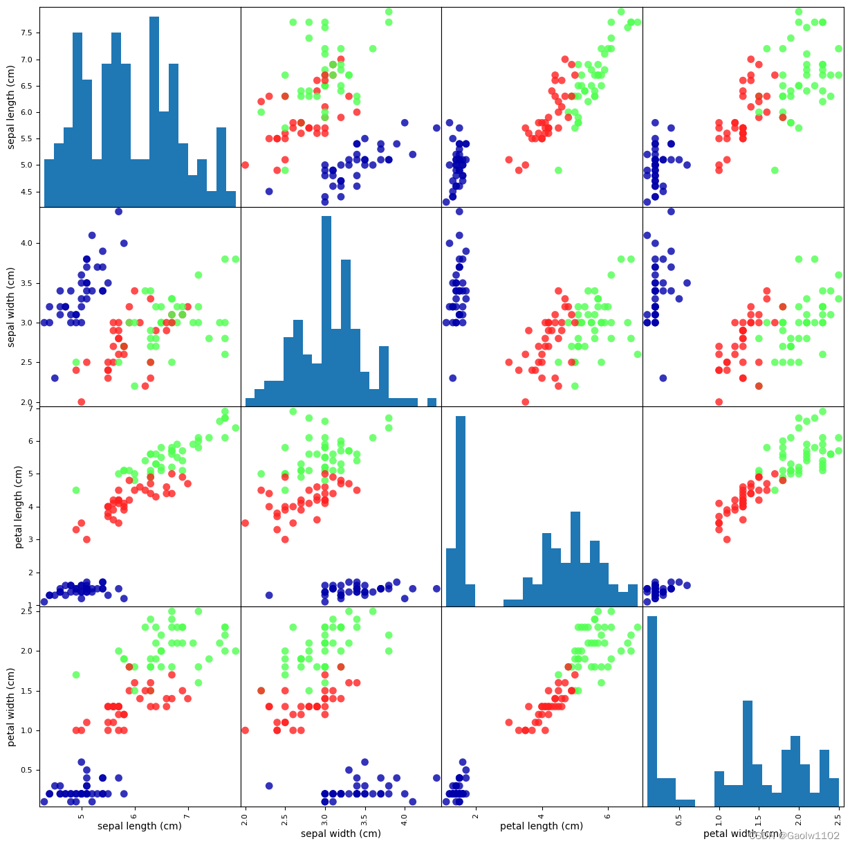
Step3：观察数据图(以pandas库生成数据图表)

import pandas as pd
import mglearn

# 利用 X_train中的数据创建 DataFrame
# 利用 iris_dataset.feature_names中的字符串对数据列进行标记
iris_dataframe = pd.DataFrame(X_train, columns=iris_dataset['feature_names'])

# 利用DataFrame创建散点图矩阵，按 y_train 着色
grr = pd.plotting.scatter_matrix(iris_dataframe, c=y_train, figsize=(15,15), marker='o',
                       hist_kwds={'bins':20}, s=60, alpha=.8, cmap=mglearn.cm3)

运行结果(根据分布特点可使用knn算法)

---

Step4：构建模型训练数据----K近邻算法

from sklearn.neighbors import KNeighborsClassifier

knn = KNeighborsClassifier(n_neighbors=1)		#设置邻点个数为 1
knn.fit(X_train, y_train)				#通过训练集构建模型

运行结果

KNeighborsClassifier(n_neighbors=1)

---

Step5：输入数据做出预测

import numpy as np
X_new = np.array([[5, 2.9, 1, 0.2]])
print('X_new shape: {}'.format(X_new.shape))

运行结果(待输入模型的数据)

X_new shape: (1, 4)

prediction = knn.predict(X_new)
print('The predict is: {}'.format(iris_dataset['target_names'][prediction]))

运行结果

The predict is: ['setosa']

预测正确

---

Step6：评估模型

y_pre = knn.predict(X_test)
print('Test set predictions:\n {}'.format(y_pre))

Test set predictions:
 [2 1 0 2 0 2 0 1 1 1 2 1 1 1 1 0 1 1 0 0 2 1 0 0 2 0 0 1 1 0 2 1 0 2 2 1 0
 2]

print(y_test)

[2 1 0 2 0 2 0 1 1 1 2 1 1 1 1 0 1 1 0 0 2 1 0 0 2 0 0 1 1 0 2 1 0 2 2 1 0
 1]

可观测得出，该两个列表仅最后一个label不同。

print('Test set score: {:.2f}'.format(np.mean(y_pre==y_test)))

手动评估结果

Test set score: 0.97

print(knn.score(X_test,y_test))

算法评估结果

0.9736842105263158