【OpenCV】OpenCV常用函数合集【持续更新】
目录1.输入、显示和保存图像2.读取、显示、保存和处理视频3.画线,画圆,画矩形,画多边形,显示文字4.框住并得到目标位置(获取鼠标消息)5.滑动条作调色板6.图像基础操作:像素、属性、ROI、通道、填充7.图像运算:加法、混合8.性能检测和优化1.输入、显示和保存图像关键函数:读取:imread()显示:imshow()保存:imwrite()窗口:namedWindow()i......
·
目录
- 1.输入、显示和保存图像
- 2.读取、显示、保存和处理视频
- 3.画线,画圆,画矩形,画多边形,显示文字
- 4.框住并得到目标位置(获取鼠标消息)
- 5.滑动条作调色板
- 6.图像基础操作:像素、属性、ROI、通道、填充
- 7.图像运算:加法、混合
- 8.性能检测和优化
- 9.颜色空间转换
- 10.图像几何变换:扩展缩放、平移、旋转、仿射变换、透视变换
- 11.图像二值化:简单阈值,自适应阈值,Otsu阈值
- 12.图像平滑:平均、高斯、中值、双边滤波
- 13.图像形态学转换
- 14.图像梯度:各种算子
- 15.图像金字塔
- 16.图像轮廓
- 17.直方图计算绘制、均衡化、反向投影、2D投影
- 18.图像变换:傅里叶变换
- 19.图像模板匹配
- 20.Hough直线变换
- 21.Hough 圆环变换
- 22.GrabCut算法进行交互式前景提取
- 23.角点检测
- 24.SIFT算法
- 25.ORB算法
1.输入、显示和保存图像
关键函数:
- 读取:imread()
- 显示:imshow()
- 保存:imwrite()
- 窗口:namedWindow()
import cv2 #引用模块
'''输入图像'''
img = cv2.imread('xxx.jpg',1)
'''显示图像'''
cv2.namedWindow('img_win',cv2.WINDOW_NORMAL)#设置一个名为img_win的窗口,窗口属性为NORMAL
cv2.imshow('img_win',img)
k = cv2.waitKey(0)
if k==27:                    #ESC
   cv2.destroyAllWindows()
elif k==ord('s') :           #按下s
    cv2.imwrite('xxx.jpg',img)    '''保存图像'''
    cv2.destroyAllWindows()
2.读取、显示、保存和处理视频
关键函数:
- VideoCapture(),参数为0为读取摄像头,参数为文件名读取对应视频文件
import cv2
'''读取摄像头'''
def CapFromCamera():
    cap = cv2.VideoCapture(0)
    while(True):
        ret, frame = cap.read()                        #读取帧
        gray = cv2.cvtColor(frame, cv2.COLOR_BGR2GRAY) #灰度化展示(简单对其进行处理)
        cv2.imshow('frame',gray)
        if cv2.waitKey(1) & 0xFF == ord('q'):          #按‘q’退出
            break
    #释放资源并关闭窗口
    cap.release()
    cv2.destroyAllWindows()
'''读取视频'''
def CapFromVedio():
    cap = cv2.VideoCapture('xxx.mp4')
    while(cap.isOpened()):
        ret, frame = cap.read()
        cv2.imshow('frame',frame)
        if cv2.waitKey(50) & 0xFF == 27:				#按ESC退出
            break
    cap.release()
    cv2.destroyAllWindows()
3.画线,画圆,画矩形,画多边形,显示文字
关键函数:
- 线:line()
- 矩形:rectangle()
- 圆:circle()
- 多边形:polylines()
- 显示文字:putText()
import cv2
import numpy as np
img=cv2.imread('fish.png',1)

# 从img的(1,1)位置,直线画到(100,100)位置,颜色BGR为(255,0,0),粗细为5
cv2.line(img,(1,1),(100,100),color=(255,0,0),thickness=5)							'''1.画线'''
cv2.rectangle(img,(10,9),(281,127),(0,255,0),5)										'''2.画矩形'''

#圆的话只需要指定半径和圆心
cv2.circle(img,(50,50),50,(0,0,255),5)												'''3.画圆'''

#画多边形
pts=np.array([[10,5],[20,30],[70,20],[50,10]], np.int32)
pts=pts.reshape((-1,1,2))
cv2.polylines(img,[pts],True,(255,255,0),3)											'''4.多边形'''

#写字
cv2.putText(img,"Hello world",(100,100),cv2.FONT_HERSHEY_SIMPLEX,4,(255,0,255),3)	'''5.显示文字'''

cv2.imshow('img',img)
cv2.waitKey(0)
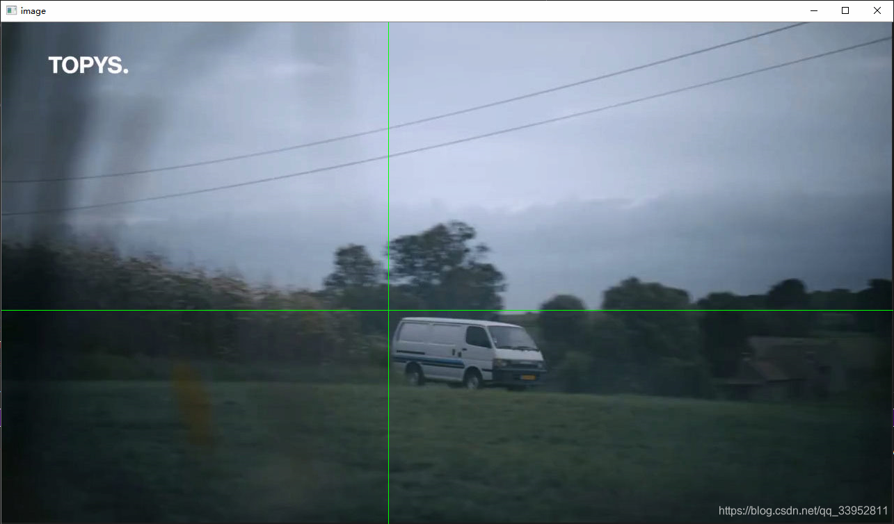
4.框住并得到目标位置(获取鼠标消息)
- setMouseCallback():回调函数,第一个参数为窗口名,需要自己设计;第二个参数为自己写的函数,在这里我写了一个可以对目标进行框定和位置获取的函数。
import cv2
# 查看鼠标支持的操作
events=[i for i in dir(cv2) if 'EVENT'in i]
print(events)
img = cv2.imread('car.png')
cv2.namedWindow('image')
#画笔
drawing_flag=True
s_x,s_y=0,0
def draw(event,x,y,flags,param):
global s_x,s_y,drawing_flag,img,img_t
if event==cv2.EVENT_MOUSEMOVE: #如果是:移动鼠标
if drawing_flag==True:
img = cv2.imread('car.png')
cv2.line(img, (x, 0), (x, img.shape[1]), color=(0, 255, 0), thickness=1)
cv2.line(img, (0, y), (img.shape[1], y), color=(0, 255, 0), thickness=1)
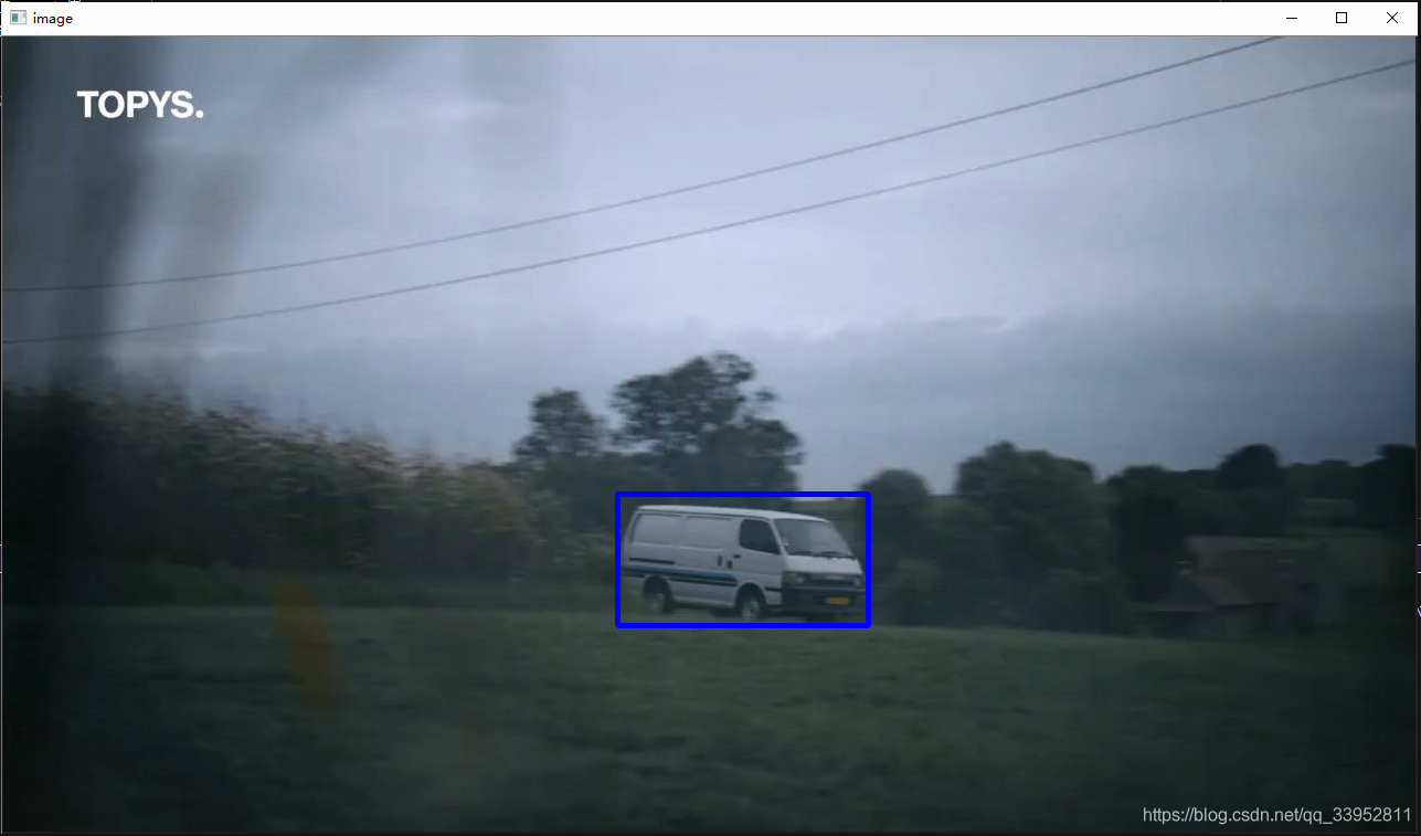
if event==cv2.EVENT_LBUTTONDOWN:#如果是:按下左键
s_x=x
s_y=y
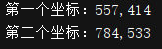
print("第一个坐标:"+str(x)+","+str(y))
elif event==cv2.EVENT_MOUSEMOVE and flags==cv2.EVENT_FLAG_LBUTTON:#如果是:移动同时左键按下
img = cv2.imread('car.png')
cv2.rectangle(img, (s_x, s_y), (x, y), (255, 0, 0), 3)
elif event==cv2.EVENT_LBUTTONUP:#如果左键松开
print("第二个坐标:" + str(x) + "," + str(y))
cv2.rectangle(img, (s_x, s_y), (x, y), (255, 0, 0), 3)
drawing_flag=False
cv2.setMouseCallback('image',draw)
while(1):
cv2.imshow('image',img)
if cv2.waitKey(10)&0xff==ord('q'):
break
cv2.destroyAllWindows()
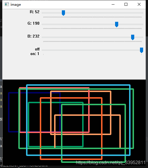
5.滑动条作调色板
- createTrackbar():创建一个滑动条
- getTrackbarPos():获取滑动条的值
import cv2
import numpy as np

drawing_flag=True
s_x,s_y=0,0

def draw_circle_2(event,x,y,flags,param):
    global s_x,s_y,drawing_flag,img
    r = cv2.getTrackbarPos('R', 'image')
    g = cv2.getTrackbarPos('G', 'image')
    b = cv2.getTrackbarPos('B', 'image')
    color = [b, g, r]
    if event==cv2.EVENT_LBUTTONDOWN:#如果是:按下左键
        s_x=x
        s_y=y
    elif event==cv2.EVENT_MOUSEMOVE  and flags==cv2.EVENT_FLAG_LBUTTON:#如果是:移动同时左键按下
        if drawing_flag==True:
            None
    elif event==cv2.EVENT_LBUTTONUP:#如果左键松开
        drawing_flag=False
        cv2.rectangle(img, (s_x, s_y), (x, y), color, 3)
    elif event==cv2.EVENT_RBUTTONDOWN:
        img = np.ones((300, 500, 3), np.uint8)

def None1():
    pass

img = np.ones((300,500,3),np.uint8)
cv2.namedWindow('image')
cv2.createTrackbar('R','image',0,255,None1)
cv2.createTrackbar('G','image',0,255,None1)
cv2.createTrackbar('B','image',0,255,None1)
switch='off\non'
cv2.createTrackbar(switch,'image',0,1,None1)

cv2.setMouseCallback('image', draw_circle_2)

while(1):
    cv2.imshow('image',img)
    k=cv2.waitKey(1)&0xFF
    if k==27:
        break

cv2.destroyAllWindows()
6.图像基础操作:像素、属性、ROI、通道、填充
- 像素:直接对原图数值进行更改
- 属性:size、dtype、shape
- ROI:感兴趣区域
- 通道:img的第三维的数值
- 填充:四周填充copyMakeBorder()
from cv2 import *
from matplotlib import pyplot as plt

img = imread('xxx.jpg',1)

# A.对老虎图片像素进行修改
#print(img) 像素
img[140:150,200:270,0:3]=0
#img[:,:,:2]=0                  #使得图像为红色
putText(img,"Hello World",(150,80),FONT_HERSHEY_SIMPLEX,2,(0,255,255),4)
imshow('img',img)

# B.获取图像属性
print("像素总数:"+str(img.size)+"\n图像数据类型:"+str(img.dtype)+"\n图像大小"+str(img.shape))

# C.图像ROI
eye = img[140:150,200:270,0:3]

# D.拆分及合并图像通道
b=img[:,:,0]
g=img[:,:,1]
r=img[:,:,2]
#或
b_,g_,r_=split(img)
#img=merge(b_,g_,r_)

#E.图像填充
BLUE=[255,0,0]
img1=imread('xxx.jpg')
replicate = copyMakeBorder(img1,10,10,10,10,BORDER_REPLICATE)
reflect = copyMakeBorder(img1,10,10,10,10,BORDER_REFLECT)
reflect101 = copyMakeBorder(img1,10,10,10,10,BORDER_REFLECT_101)
wrap = copyMakeBorder(img1,10,10,10,10,BORDER_WRAP)
constant= copyMakeBorder(img1,10,10,10,10,BORDER_CONSTANT,value=BLUE)
plt.subplot(231),plt.imshow(img1,'gray'),plt.title('ORIGINAL')
plt.subplot(232),plt.imshow(replicate,'gray'),plt.title('REPLICATE')
plt.subplot(233),plt.imshow(reflect,'gray'),plt.title('REFLECT')
plt.subplot(234),plt.imshow(reflect101,'gray'),plt.title('REFLECT_101')
plt.subplot(235),plt.imshow(wrap,'gray'),plt.title('WRAP')
plt.subplot(236),plt.imshow(constant,'gray'),plt.title('CONSTANT')
plt.show()

waitKey(0)
7.图像运算:加法、混合
关键函数:
- 相加:add()
- 混合:addWeighted(),参数4和参数3表示参数3和参数1的混合比例
import cv2
import numpy as np
# 1.加法
img=np.zeros((500,500,1),np.uint8)
color = np.ones((500,500,1),np.uint8)
print(cv2.add(img,color))

# 2.混合
img1=cv2.imread('building01.jpg')
img = cv2.imread('xxx.jpg')
img  =cv2.resize(img,(384,288))
dst=cv2.addWeighted(img1,0.7,img,0.5,0)
cv2.imshow('dst',dst)
cv2.waitKey(0)
8.性能检测和优化
关键函数:
- 获取时间点:getTickCount()
- 设置优化:setUseOptimized()
from cv2 import *

# 检测时间
e1=getTickCount()
'''
Code
'''
e2=getTickCount()
time=(e2-e1)/getTickFrequency()
print(time)

# 检测优化、开启优化
print(useOptimized())
setUseOptimized(False)
print(useOptimized())
setUseOptimized(True)
print(useOptimized())

'''
优化建议:
1. 尽量避免使用循环,尤其双层三层循环,它们天生就是非常慢的。
2. 算法中尽量使用向量操作,因为 Numpy 和 OpenCV 都对向量操作进行
了优化。
3. 利用高速缓存一致性。
4. 没有必要的话就不要复制数组。使用视图来代替复制。数组复制是非常浪
费资源的。
'''
9.颜色空间转换
关键函数:
- 颜色空间转换:cvtColor()
- 判断像素值是否在某区间:inrange()
import cv2

img = cv2.imread('xxx.png')
# 参数1:img_name	参数2:flag(还有其他类型的转换)
cv2.cvtColor(img,cv2.COLOR_BGR2GRAY)		#将BGR颜色空间转换为GRAY(灰度化)
# hsv,mask_1
lower_ = np.array([0, 0,100])
upper_ = np.array([120 , 50, 240])
hsv = cv2.cvtColor(final, cv2.COLOR_BGR2HSV)#转换为HSV
mask_1 = cv2.inRange(hsv, lower_, upper_)	#HSV在lower_到upper_的为255,否则设置为0
备注:可以利用这个方法,找到自己感兴趣的物体,从而进行跟踪
10.图像几何变换:扩展缩放、平移、旋转、仿射变换、透视变换
关键函数:
- 扩展缩放:resize()
- 仿射变换:warpAffine()
- 旋转辅助函数:getRotationMatrix2D()
- 透视变换:getPerspectiveTransform(),warpPerspective()
import cv2
import numpy as np
img = cv2.imread('xxx.jpg')


#缩放,推荐cv2.INTER_AREA,扩展推荐v2.INTER_CUBIC,cv2.INTER_LINEAR,默认cv2.INTER_LINEAR
'''resize函数'''
res=cv2.resize(img,None,fx=0.5,fy=0.5,interpolation=cv2.INTER_LINEAR)

#平移
'''warpAffine函数,接收2x3矩阵,前两列固定,后两列是平移长度'''
Mat = np.float32([[1,0,100],[0,1,50]])
res2=cv2.warpAffine(img,Mat,(300,300))

#旋转
# 这里的第一个参数为旋转中心,第二个为旋转角度,第三个为旋转后的缩放因子
# 可以通过设置旋转中心,缩放因子,以及窗口大小来防止旋转后超出边界的问题
'''getRotationMatrix2D函数,接收3x3矩阵'''
rows,cols=img.shape[:2]
M=cv2.getRotationMatrix2D((cols/2,rows/2),45,0.6)
res3=cv2.warpAffine(img,M,(300,300))

#仿射变换
'''getAffineTransform()函数,图像前的三个点,图像后的三个点,形成仿射变换'''
pts1=np.float32([[50,50],[150,50],[50,200]])
pts2=np.float32([[10,100],[50,50],[50,250]])
M1=cv2.getAffineTransform(pts1,pts2)
res4=cv2.warpAffine(img,M1,(cols,rows))

#透视变换
'''getPerspectiveTransform()函数,需要2个参数,图像前4个点,图像后4个点,一般用来矫正图像'''
img2=cv2.imread('xxx.jpg')
res5=cv2.resize(img2,None,fx=0.2,fy=0.2)
rows,cols,ch=img2.shape
pts3 = np.float32([[56,65],[368,52],[28,387],[389,390]])
pts4 = np.float32([[0,0],[300,0],[0,300],[300,300]])
M2=cv2.getPerspectiveTransform(pts3,pts4)
res5=cv2.warpPerspective(res5,M2,(800,800))

while(1):
    cv2.imshow('src', img)
    cv2.imshow('res1',res)
    cv2.imshow('res2',res2)
    cv2.imshow('res3',res3)
    cv2.imshow('res4',res4)
    cv2.imshow('res5',res5)
    if cv2.waitKey(1) & 0xFF==27:
        break
11.图像二值化:简单阈值,自适应阈值,Otsu阈值
关键函数:
- 阈值分割:threshold()
- 自适应阈值:adaptiveThreshold()
import cv2
img = cv2.imread('xxx.png',0)

# 简单阈值
# 第四个参数可更改
ret,thread=cv2.threshold(img,126,245,cv2.THRESH_BINARY)
'''自适应阈值'''
img = cv2.medianBlur(img,5)
ret,th1 = cv2.threshold(img,127,255,cv2.THRESH_BINARY)
#11 为 Block size, 2 为 C 值
th2 = cv2.adaptiveThreshold(img,255,cv2.ADAPTIVE_THRESH_MEAN_C,\
cv2.THRESH_BINARY,11,2)
'''OTSU阈值'''
ret3,th3 = cv2.threshold(img,0,255,cv2.THRESH_BINARY+cv2.THRESH_OTSU)
while(1):
    cv2.imshow('src',img)
    cv2.imshow('img_th1',thread)
    cv2.imshow('img_th2',th2)
    cv2.imshow('img_th3',th3)
    if cv2.waitKey(1)& 0xFF==27:
        break
12.图像平滑:平均、高斯、中值、双边滤波
关键函数:
- 滤波:blur()
- 高斯滤波:GaussianBlur()
- 中值滤波:medianBlur()
- 双边滤波:bilateralFilter()
import cv2
from matplotlib import pyplot as plt
img = cv2.imread('xxx.jpg')

#均值
blur= cv2.blur(img,(5,5))
plt.subplot(121),plt.imshow(img),plt.title('src'),plt.xticks([]),plt.yticks([])
plt.subplot(122),plt.imshow(blur),plt.title('blur'),plt.xticks([]),plt.yticks([])

#高斯
Gaussi=cv2.GaussianBlur(img,(5,5),0)
plt.subplot(122),plt.imshow(Gaussi),plt.title('Gaussian'),plt.xticks([]),plt.yticks([])

#中值滤波
median = cv2.medianBlur(img,5)
plt.subplot(122),plt.imshow(median),plt.title('median'),plt.xticks([]),plt.yticks([])

#双边滤波
bilateralFilter = cv2.bilateralFilter(img,9,75,75)
plt.subplot(122),plt.imshow(bilateralFilter),plt.title('bilateralFilter'),plt.xticks([]),plt.yticks([])

plt.show()
13.图像形态学转换
关键函数:
- 腐蚀、膨胀、开闭、梯度、礼帽黑帽详见代码
import cv2
import numpy as np

img = cv2.imread('xxx.png',0)
kernel = np.ones((17,17),np.uint8)
# 腐蚀
test1 = cv2.erode(img,kernel=kernel)
# 膨胀
test2 = cv2.dilate(img,kernel=kernel)
# 开运算
test3 = cv2.morphologyEx(img,cv2.MORPH_OPEN,kernel=kernel)
# 闭运算
test4 = cv2.morphologyEx(img,cv2.MORPH_OPEN,kernel=kernel)
# 形态学梯度 膨胀-腐蚀
gradient = cv2.morphologyEx(img, cv2.MORPH_GRADIENT, kernel)
# 礼帽 原始图像与进行开运算之后得到的图像的差。
tophat = cv2.morphologyEx(img, cv2.MORPH_TOPHAT, kernel)
# 黑帽 进行闭运算之后得到的图像与原始图像的差
blackhat = cv2.morphologyEx(img, cv2.MORPH_BLACKHAT, kernel)
while(1):
    cv2.imshow('src',img)
    cv2.imshow('test1',test1)
    cv2.imshow('test2',test2)
    cv2.imshow('test3', test3)
    cv2.imshow('test4',test4)
    cv2.imshow('gradient',gradient)
    cv2.imshow('test6',tophat)
    cv2.imshow('test7',blackhat)
    if cv2.waitKey(0) & 0xFF==27:
        break
14.图像梯度:各种算子
常见算子:
- 拉普拉斯: Laplacian()
- Sobel算子:Sobel()
- Canny算子:Canny()
import cv2
img=cv2.imread('XT.png',0)
#cv2.CV_64F 输出图像的深度(数据类型),可以使用-1, 与原图像保持一致 np.uint8
laplacian=cv2.Laplacian(img,cv2.CV_64F)
# 参数 1,0 为只在 x 方向求一阶导数,最大可以求 2 阶导数。
sobelx=cv2.Sobel(img,cv2.CV_64F,1,0,ksize=3) # 参数 0,1 为只在 y 方向求一阶导数,最大可以求 2 阶导数。
sobely=cv2.Sobel(img,cv2.CV_64F,0,1,ksize=3)
Canny = cv2.Canny(img,100,240)
while(1):
    cv2.imshow('src',img)
    cv2.imshow('laplacian',laplacian)
    cv2.imshow('sobelx',sobelx)
    cv2.imshow('sobely', sobely)
    cv2.imshow('Canny',Canny)
    if cv2.waitKey(0) & 0xFF==27:
        break
15.图像金字塔
关键函数:
- pyrDown()
- pyrUp()
import cv2
img = cv2.imread('xxx.jpg')
lower_reso = cv2.pyrDown(img)
high_reso = cv2.pyrUp(lower_reso)
cv2.imshow('img',high_reso)
cv2.waitKey(0)
16.图像轮廓
主要函数:
- 找轮廓 findContours
- 画轮廓 drawContours
其他:重心、周长、面积、轮廓近似、凸包、矩阵、最小外接圆、椭圆和直线拟合
from cv2 import *

img = imread('dog2.jpg',0)
imshow('img',img)

#绘制轮廓
ret,threah = threshold(img,127,255,0)
image, contours, hierarchy = findContours(threah,RETR_TREE,CHAIN_APPROX_NONE)
res= drawContours(img,contours,-1,(255,100,0),3)

imshow('threah',threah)
imshow('res',res)

cnt = contours[2]
M = moments(cnt)
#print(M)
#重心
cx = int(M['m10']/M['m00'])
cy = int(M['m01']/M['m00'])
# print(cx,cy)
#面积
area = contourArea(cnt)
# print(area)
#周长
perimeter = arcLength(cnt,True)
#print(perimeter)
#轮廓近似
epsilon = 0.1*arcLength(cnt,True)
approx = approxPolyDP(cnt,epsilon,True)
#凸包
hull = convexHull(cnt)
#凸性检测
k = isContourConvex(cnt)#False说明不是凸性
#print(k)

#直矩阵
x,y,w,h = boundingRect(cnt)
img = rectangle(img,(x,y),(x+w,y+h),(100,255,0),3)
imshow('img_b',img)
#旋转矩阵
x,y,w,h = boundingRect(cnt)
img = rectangle(img,(x,y),(x+w,y+h),(100,255,0),2)
#imshow('img_c',img)
#最小外接圆
(x,y),radius = minEnclosingCircle(cnt)
center = (int(x),int(y))#cv2.namedWindow('image')
radius = int(radius)
img = circle(img,center,radius,(100,240,0),2)
#imshow('img_r',img)
# 椭圆拟合
ellipse = fitEllipse(cnt)
img = ellipse(img,ellipse,(0,255,0),2)
# imshow('img_i',img)
#直线拟合
cols=img.shape[1]
[vx,vy,x,y] = fitLine(cnt, cv2.DIST_L2,0,0.01,0.01)
lefty = int((-x*vy/vx) + y)
righty = int(((cols-x)*vy/vx)+y)
img = line(img,(cols-1,righty),(0,lefty),(0,255,0),2)

#print(hull)
waitKey(0)
17.直方图计算绘制、均衡化、反向投影、2D投影
关键函数:
- 计算直方图:calcHist()
- 绘制直方图(pyplot):hist()
- 直方图均衡化:equalizeHist()
import cv2
import numpy as np
from matplotlib import pyplot as plt
img = cv2.imread('xxx.jpg',0)
cv2.imshow('xxx',img)

'''1.计算直方图'''
# 输入表示:原图、通道、Mask、BIN数目,范围
'''返回的参数hist是一个1x256的一维数组'''
hist = cv2.calcHist([img],[0],None,[256],[0,256])
print(hist)
#或者是np中的histogram来进行直方图的运算
#hist,bins = np.histogram(img.ravel(),256,[0,256])

'''2.绘制直方图'''
#这里可以使用matplotlib方式进行绘制,比较简单
plt.hist(img.ravel(),256,[0,256])
plt.show()

'''小实验A,绘制三通道彩色图'''
img = cv2.imread('xxx.jpg')
bgr=['b','g','r']
for i,color in enumerate(bgr):
    hist = cv2.calcHist([img],[i],None,[256],[0,256])
    plt.plot(hist,color=color)
    plt.xlim([0,256])
cv2.imshow('img',img)
plt.show()

'''小实验B,利用numpy进行掩膜运算得到直方图'''
mask = np.zeros(img.shape[:2],np.uint8)
mask[100:200,300:400]=255
mask_img = cv2.bitwise_and(img,img,mask)
hist_full = cv2.calcHist([img],[0],None,[256],[0,256])
hist_mask = cv2.calcHist([img],[0],mask,[256],[0,256])
plt.subplot(221), plt.imshow(img, 'gray')
plt.subplot(222), plt.imshow(mask,'gray')
plt.subplot(223), plt.imshow(mask_img, 'gray')
plt.subplot(224), plt.plot(hist_full), plt.plot(hist_mask)
plt.xlim([0,256])
plt.show()

'''3.直方图均衡化'''
# img_3= cv2.imread('xxx.jpg')
# hist , bins= np.histogram(img_3.flatten(),256,[0,256])#flagtten函数可以将img_3转为一维
# #计算累计直方图
# cdf = hist.cumsum()
# cdf_normalized = cdf * hist.max()/ cdf.max()
# plt.plot(cdf_normalized, color = 'b')
# plt.hist(img.flatten(),256,[0,256], color = 'r')
# plt.xlim([0,256])
# plt.legend(('cdf','histogram'), loc = 'upper left')
# plt.show()
# # 构建 Numpy 掩模数组,cdf 为原数组,当数组元素为 0 时,掩盖(计算时被忽略)。
# cdf_m = np.ma.masked_equal(cdf,0)
# cdf_m = (cdf_m - cdf_m.min())*255/(cdf_m.max()-cdf_m.min())
# # 对被掩盖的元素赋值,这里赋值为 0
# cdf = np.ma.filled(cdf_m,0).astype('uint8')
# img_3_1=cdf[img_3]
img = cv2.imread('xxx.jpg',0)
equ = cv2.equalizeHist(img)
res = np.hstack((img,equ))
cv2.imshow('res.png',res)

clahe = cv2.createCLAHE(clipLimit=2.0, tileGridSize=(8,8))
cl1 = clahe.apply(img)
res2 = np.hstack((img,cl1))
cv2.imshow('res1.png',res2)

'''4.2D直方图'''
#如果要绘制颜色直方图,需要将图像的颜色空间从BGR转换到HSV
#计算以为直方图,要从BGR转为HSV
img = cv2.imread('xxx.jpg')
hsv=cv2.cvtColor(img,cv2.COLOR_BGR2HSV)
#channels为H、S两个通道,H通道为180,S通道为256
#取值范围H通道从0到180,S通道为0到256
hist =  cv2.calcHist([hsv],[0,1],None,[180,256],[0,180,0,256])
#numpy中也有相关函数,histogram2d
#绘制直方图
plt.imshow(hist,interpolation='nearest')
plt.show()

'''5.直方图反向投影'''
# 直方图反向投影经常与图像分割密切联系
roi = cv2.imread('xxx_roi.png')
hsv = cv2.cvtColor(roi,cv2.COLOR_BGR2HSV)
target = cv2.imread('xxx.jpg')
hsvt = cv2.cvtColor(target,cv2.COLOR_BGR2HSV)
roihist = cv2.calcHist([hsv],[0, 1], None, [180, 256], [0, 180, 0, 256] )
# 归一化:原始图像,结果图像,映射到结果图像中的最小值,最大值,归一化类型
#cv2.NORM_MINMAX 对数组的所有值进行转化,使它们线性映射到最小值和最大值之间
# 归一化之后的直方图便于显示,归一化之后就成了 0 到 255 之间的数了。
cv2.normalize(roihist,roihist,0,255,cv2.NORM_MINMAX)
dst = cv2.calcBackProject([hsvt],[0,1],roihist,[0,180,0,256],1) # Now convolute with circular disc
# 此处卷积可以把分散的点连在一起
disc = cv2.getStructuringElement(cv2.MORPH_ELLIPSE,(5,5))
dst=cv2.filter2D(dst,-1,disc)
# threshold and binary AND
ret,thresh = cv2.threshold(dst,50,255,0) # 别忘了是三通道图像,因此这里使用 merge 变成 3 通道
thresh = cv2.merge((thresh,thresh,thresh))
# 按位操作
res = cv2.bitwise_and(target,thresh)
res = np.hstack((target,thresh,res))
# 显示图像
cv2.imshow('1',res)
cv2.waitKey(0)
18.图像变换:傅里叶变换
- 快速傅里叶变换(np):fft()
- 傅里叶变换(opencv):dft()
'''边界和噪声是图像中的高频分量'''
'''可以通过高频分量的分布来消除噪声点等'''
'''振幅谱是一个波或波列的振幅随频率的变化关系'''
import cv2
import numpy as np
from matplotlib import pyplot as plt

img = cv2.imread('xxx.jpg',0)
f = np.fft.fft2(img)
fshift = np.fft.fftshift(f)
# 这里构建振幅图的公式没学过
magnitude_spectrum = 20*np.log(np.abs(fshift))
plt.subplot(121),plt.imshow(img, cmap = 'gray')
plt.title('Input Image'), plt.xticks([]), plt.yticks([])
plt.subplot(122),plt.imshow(magnitude_spectrum, cmap = 'gray')
# 振幅谱
plt.title('Magnitude Spectrum'), plt.xticks([]), plt.yticks([])
plt.show()

rows, cols = img.shape
crow,ccol = int(rows/2) , int(cols/2)
print(crow,ccol)
fshift[crow-30:crow+30, ccol-30:ccol+30] = 0
f_ishift = np.fft.ifftshift(fshift)
img_back = np.fft.ifft2(f_ishift)
# 取绝对值
img_back = np.abs(img_back)
plt.subplot(131),plt.imshow(img, cmap = 'gray')
plt.title('Input Image'), plt.xticks([]), plt.yticks([])
plt.subplot(132),plt.imshow(img_back, cmap = 'gray')
plt.title('Image after HPF'), plt.xticks([]), plt.yticks([])
plt.subplot(133),plt.imshow(img_back)
plt.title('Result in JET'), plt.xticks([]), plt.yticks([])
plt.show()

#opencv中的傅里叶变换
img = cv2.imread('xxx.jpg',0)
dft = cv2.dft(np.float32(img),flags = cv2.DFT_COMPLEX_OUTPUT)
dft_shift = np.fft.fftshift(dft)
magnitude_spectrum = 20*np.log(cv2.magnitude(dft_shift[:,:,0],dft_shift[:,:,1]))
plt.subplot(121),plt.imshow(img, cmap = 'gray')
plt.title('Input Image'), plt.xticks([]), plt.yticks([])
plt.subplot(122),plt.imshow(magnitude_spectrum, cmap = 'gray')
plt.title('Magnitude Spectrum'), plt.xticks([]), plt.yticks([])
plt.show()
# 高通滤波,如拉普拉斯算子
rows, cols = img.shape
crow,ccol = int(rows/2) , int(cols/2)
mask = np.zeros((rows,cols,2),np.uint8)
mask[crow-30:crow+30, ccol-30:ccol+30] = 1
# apply mask and inverse DFT
fshift = dft_shift*mask
f_ishift = np.fft.ifftshift(fshift)
img_back = cv2.idft(f_ishift)
img_back = cv2.magnitude(img_back[:,:,0],img_back[:,:,1])
plt.subplot(121),plt.imshow(img, cmap = 'gray')
plt.title('Input Image'), plt.xticks([]), plt.yticks([])
plt.subplot(122),plt.imshow(img_back, cmap = 'gray')
plt.title('Magnitude Spectrum'), plt.xticks([]), plt.yticks([])
plt.show()
19.图像模板匹配
关键函数:
- 模板匹配:matchTemplate()
import cv2
import numpy as np
from matplotlib import pyplot as plt
#单目标
img = cv2.imread('xxx.jpg',0)
img2 = img.copy()
template = cv2.imread('xxx_roi.png',0)
w, h = template.shape[::-1]
# 6中匹配的方式
methods = ['cv2.TM_CCOEFF', 'cv2.TM_CCOEFF_NORMED', 'cv2.TM_CCORR',
'cv2.TM_CCORR_NORMED', 'cv2.TM_SQDIFF', 'cv2.TM_SQDIFF_NORMED']
for meth in methods:
img = img2.copy()
method = eval(meth)
res = cv2.matchTemplate(img,template,method)
#cv2.imshow('imshow',res)
min_val, max_val, min_loc, max_loc = cv2.minMaxLoc(res)
#print(min_val,max_val,min_loc,max_loc)
# 使用不同的比较方法,对结果的解释不同
# If the method is TM_SQDIFF or TM_SQDIFF_NORMED, take minimum
if method in [cv2.TM_SQDIFF, cv2.TM_SQDIFF_NORMED]:
top_left = min_loc
else:
top_left = max_loc
bottom_right = (top_left[0] + w, top_left[1] + h)
cv2.rectangle(img,top_left, bottom_right, 255, 2)
plt.subplot(121),plt.imshow(res,cmap = 'gray')
plt.title('Matching Result'), plt.xticks([]), plt.yticks([])
plt.subplot(122),plt.imshow(img,cmap = 'gray')
plt.title('Detected Point'), plt.xticks([]), plt.yticks([])
plt.suptitle(meth)
plt.show()
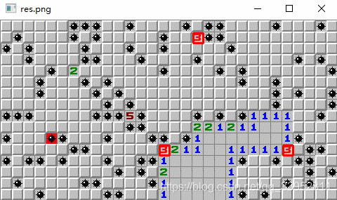
#多目标
img_rgb = cv2.imread('cut.jpg')
img_gray = cv2.cvtColor(img_rgb, cv2.COLOR_BGR2GRAY)
template = cv2.imread('3_.png',0)
w, h = template.shape[::-1]
res = cv2.matchTemplate(img_gray,template,cv2.TM_CCOEFF_NORMED)
threshold = 0.8
loc = np.where( res >= threshold)
for pt in zip(*loc[::-1]):
cv2.rectangle(img_rgb, pt, (pt[0] + w, pt[1] + h), (0,0,255), 2)
cv2.imshow('res.png',img_rgb)
cv2.waitKey(0)
多目标匹配:扫雷中“3”的个数
20.Hough直线变换
关键函数:
HoughLines():详见代码
import cv2
import numpy as np
img = cv2.imread('xxx.jpg')
gray = cv2.cvtColor(img,cv2.COLOR_BGR2GRAY)
edges = cv2.Canny(gray,50,150,apertureSize = 3)

'''方式1'''
#第二、三个值是p和setae的精确度
lines = cv2.HoughLines(edges,1,np.pi/180,200)
for i in range(0,lines.shape[0]):
    for rho,theta in lines[i]:
        a = np.cos(theta)
        b = np.sin(theta)
        x0 = a*rho
        y0 = b*rho
        x1 = int(x0 + 1000*(-b))
        y1 = int(y0 + 1000*(a))
        x2 = int(x0 - 1000*(-b))
        y2 = int(y0 - 1000*(a))
        cv2.line(img,(x1,y1),(x2,y2),(0,0,255),2)
        cv2.imshow('houghlines.jpg',img)
        cv2.waitKey(0)

'''方式2'''
#Probabilistic Hough Transform局部化霍夫变换
img = cv2.imread('xxx.jpg')
#img = cv2.resize(img,None,fx=0.2,fy=0.2)
gray = cv2.cvtColor(img,cv2.COLOR_BGR2GRAY)
edges = cv2.Canny(gray,50,150,apertureSize = 3)
minLineLength = 100
maxLineGap = 10
lines = cv2.HoughLinesP(edges,1,np.pi/180,100,minLineLength,maxLineGap)
for i in range(0,lines.shape[0]):
    for x1,y1,x2,y2 in lines[i]:
        cv2.line(img,(x1,y1),(x2,y2),(0,255,0),2)
        cv2.imshow('img',img)
        cv2.waitKey(0)
21.Hough 圆环变换
关键函数:
HoughCircles():详见代码
import cv2
import numpy as np
img = cv2.imread('circle.jpg',0)
img = cv2.medianBlur(img,5)
cimg = cv2.cvtColor(img,cv2.COLOR_GRAY2BGR)
circles = cv2.HoughCircles(img,cv2.HOUGH_GRADIENT,1,20,
param1=50,param2=30,minRadius=0,maxRadius=0)
circles = np.uint16(np.around(circles))
print(circles.shape)
for i in circles[0,:]:
    cv2.circle(cimg,(i[0],i[1]),i[2],(0,255,0),2)
    cv2.circle(cimg,(i[0],i[1]),2,(0,0,255),3)
cv2.imshow('detected circles',cimg)
cv2.waitKey(0)
cv2.destroyAllWindows()
22.GrabCut算法进行交互式前景提取
关键函数:
grabCut():详见函数
import numpy as np
import cv2
from matplotlib import pyplot as plt
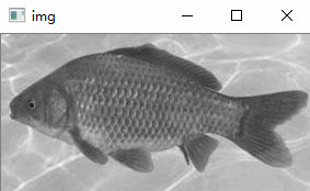
img = cv2.imread('fish.png')
cv2.imshow('img',img)
mask = np.zeros(img.shape[:2],np.uint8)
bgdModel = np.zeros((1,65),np.float64)
fgdModel = np.zeros((1,65),np.float64)
rect = (1,1,283,129) # 函数的返回值是更新的 mask, bgdModel, fgdModel
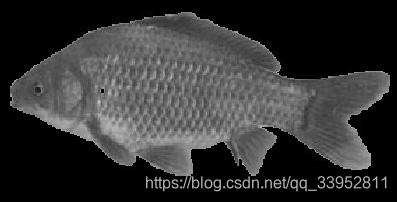
cv2.grabCut(img,mask,rect,bgdModel,fgdModel,5,cv2.GC_INIT_WITH_RECT)
mask2 = np.where((mask==2)|(mask==0),0,1).astype('uint8')
img = img*mask2[:,:,np.newaxis]
plt.imshow(img),plt.colorbar(),plt.show()
'''或者使用mask方法,这样可以使之优化'''
cv2.waitKey(0)
原图:
提取后:
23.角点检测
关键函数:
- 角点检测:cornerHarris()
- 获得n个最佳角点:goodFeaturesToTrack()
import cv2
import numpy as np
from matplotlib import pyplot as plt
img = cv2.imread('xxx.png')
gray = cv2.cvtColor(img,cv2.COLOR_BGR2GRAY)
gray = np.float32(gray)
# 输入图像必须是 float32,点大小,点偏离,
dst = cv2.cornerHarris(gray,2,3,0.05)
dst = cv2.dilate(dst,None)
img[dst>0.01*dst.max()]=[0,0,255]
cv2.imshow('dst',img)
cv2.waitKey(0)
#亚像素级精确度的角点
#得到N个最佳角点
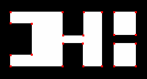
img = cv2.imread('xxx.png')
gray = cv2.cvtColor(img,cv2.COLOR_BGR2GRAY)
#质量水平在0到1之间,4表示4个点
corners = cv2.goodFeaturesToTrack(gray,4,0.01,10) # 返回的结果是 [[ 311., 250.]] 两层括号的数组。
print(corners)
corners = np.int0(corners)
print(corners)
for i in corners:
x,y = i.ravel()
cv2.circle(img,(x,y),3,255,-1)
plt.imshow(img)
plt.show()
24.SIFT算法
使用函数要版权,所以可能用不了,另外,SURF,FAST也是需要版权的,我们只需要知道它的大致原理,还有其使用场景,SIFT算法利用了尺度不变性来进行图像关键点的提取,细节原理可参考其他资料
'''SIFT算法'''
import cv2
import numpy as np
# img = cv2.imread('rice.jpg')
# gray= cv2.cvtColor(img,cv2.COLOR_BGR2GRAY)
# sift = cv2.SIFT()
# kp = sift.detect(gray,None)
# img=cv2.drawKeypoints(gray,kp)
# cv2.imwrite('sift_keypoints.jpg',img)
'''
*****步骤******
尺度空间极值检测
关键点(极值点)定位
为关键点(极值点)指定方向参数
关键点描述符
关键点匹配
**************
'''
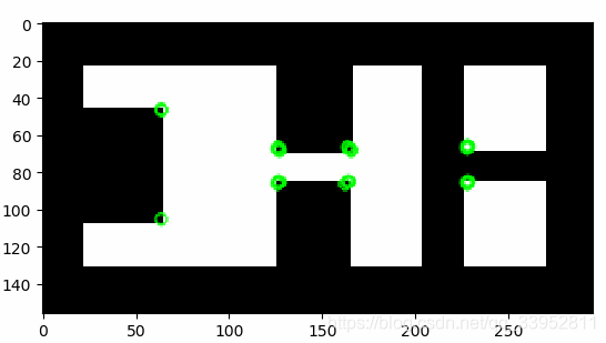
25.ORB算法
ORB是开源的,另外,利用SIFT,ORB算法等一般进行特征匹配
import cv2
from matplotlib import pyplot as plt
img = cv2.imread('XT.png',0)
# Initiate STAR detector
orb = cv2.ORB_create()
# find the keypoints with ORB
kp = orb.detect(img,None)
# compute the descriptors with ORB
kp, des = orb.compute(img, kp)
img2 = img.copy()
# draw only keypoints location,not size and orientation
img2 = cv2.drawKeypoints(img,kp,img2,color=(0,255,0), flags=0)
plt.imshow(img2),plt.show()

为开发者提供学习成长、分享交流、生态实践、资源工具等服务,帮助开发者快速成长。
更多推荐


 66
66 0
0- 0


 已为社区贡献4条内容

所有评论(0)