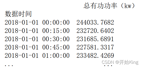
时间序列就是以时间为索引的数据，比如下面这种形式
数据链接：https://pan.baidu.com/s/1KHmCbk9ygIeRHn97oeZVMg
提取码：s0k5

python使用ARIMA建模，主要是使用statsmodels库

首先是建模流程，如果不是太明白不用担心，下面会详细的介绍这些过程

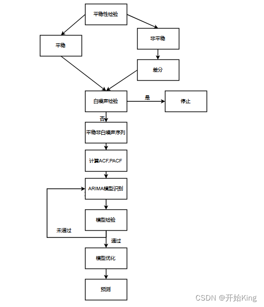
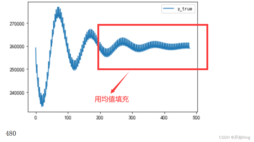
首先要注意一点，ARIMA适用于短期 单变量预测，长期的预测值都会用均值填充，后面你会看到这种情况。

首先导入需要的包

import pandas as pd
import numpy as np
import matplotlib.pyplot as plt
import statsmodels.api as sm
from statsmodels.stats.diagnostic import acorr_ljungbox
from statsmodels.graphics.tsaplots import plot_pacf,plot_acf

载入数据

df=pd.read_csv('./附件1-区域15分钟负荷数据.csv',parse_dates=['数据时间'])
df.info()

将默认索引改为时间索引

data=df.copy()
data=data.set_index('数据时间')

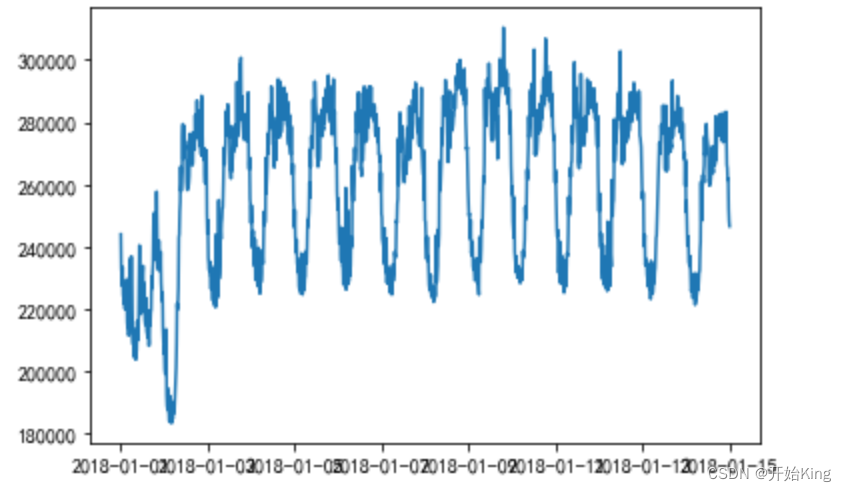
1 绘制时序图

plt.plot(data.index,data['总有功功率（kw）'].values)
plt.show()

划分训练集和测试集

train=data.loc[:'2018/1/13 23:45:00',:]
test=data.loc['2018/1/14 0:00:00':,:]

2 平稳性检验

# 单位根检验-ADF检验
print(sm.tsa.stattools.adfuller(train['总有功功率（kw）']))

1%、%5、%10不同程度拒绝原假设的统计值和ADF比较，ADF同时小于1%、5%、10%即说明非常好地拒绝该假设，本数据中，adf结果为-5.22， 小于三个level的统计值，说明数据是平稳的
3 白噪声检验
使用$Q_{BP}$ 和$Q_{LB}$ 统计量进行序列的随机性检验

# 白噪声检验
acorr_ljungbox(train['总有功功率（kw）'], lags = [6, 12],boxpierce=True)

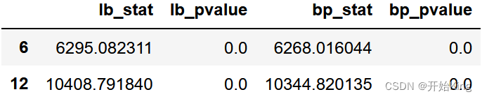各阶延迟下LB和BP统计量的P值都小于显著水平（$\alpha =0.05$）,所以拒绝序列为纯随机序列的原假设，认为该序列为非白噪声序列
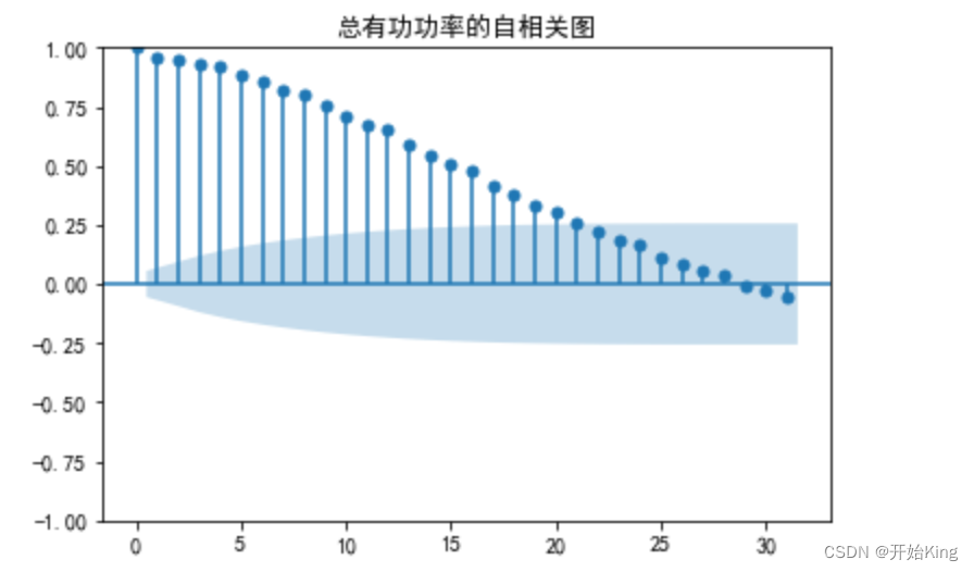
4 计算ACF,PACF

# 计算ACF
acf=plot_acf(train['总有功功率（kw）'])
plt.title("总有功功率的自相关图")
plt.show()

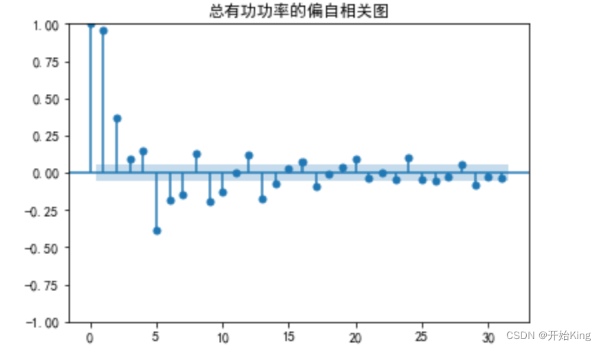
# PACF
pacf=plot_pacf(train['总有功功率（kw）'])
plt.title("总有功功率的偏自相关图")
plt.show()

5 选择合适的模型进行拟合

ACF	PACF	模型
拖尾	截尾	AR
截尾	拖尾	MA
拖尾	拖尾	ARMA

如果说自相关图拖尾，并且偏自相关图在p阶截尾时，此模型应该为AR(p )。
如果说自相关图在q阶截尾并且偏自相关图拖尾时，此模型应该为MA(q)。
如果说自相关图和偏自相关图均显示为拖尾，那么可结合ACF图中最显著的阶数作为q值，选择PACF中最显著的阶数作为p值，最终建立ARMA(p,q)模型。

从ACF和PACF图的结果来看，p=7,q=4

model = sm.tsa.arima.ARIMA(train,order=(7,0,4))
arima_res=model.fit()
arima_res.summary()

因为看自相关图和偏自相关图有很大的主观性，因此，可以通过AIC或BIC来确定最合适的阶数

trend_evaluate = sm.tsa.arma_order_select_ic(train, ic=['aic', 'bic'], trend='n', max_ar=20,
                                            max_ma=5)
print('train AIC', trend_evaluate.aic_min_order)
print('train BIC', trend_evaluate.bic_min_order)

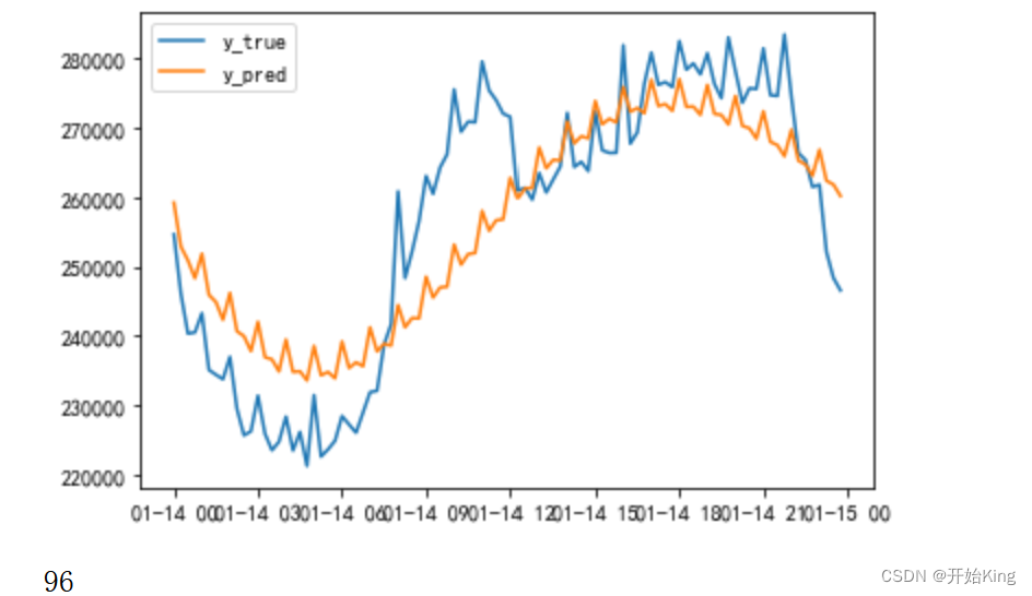
6 模型预测

predict=arima_res.predict("2018/1/14 0:00:00","2018/1/14 23:45:00")
plt.plot(test.index,test['总有功功率（kw）'])
plt.plot(test.index,predict)
plt.legend(['y_true','y_pred'])
plt.show()
print(len(predict))

7 模型评价

from sklearn.metrics import r2_score,mean_absolute_error
mean_absolute_error(test['总有功功率（kw）'],predict)

8 残差分析

res=test['总有功功率（kw）']-predict
residual=list(res)
plt.plot(residual)

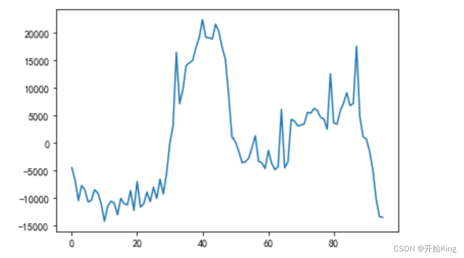
查看残差的均值是否在0附近

np.mean(residual)

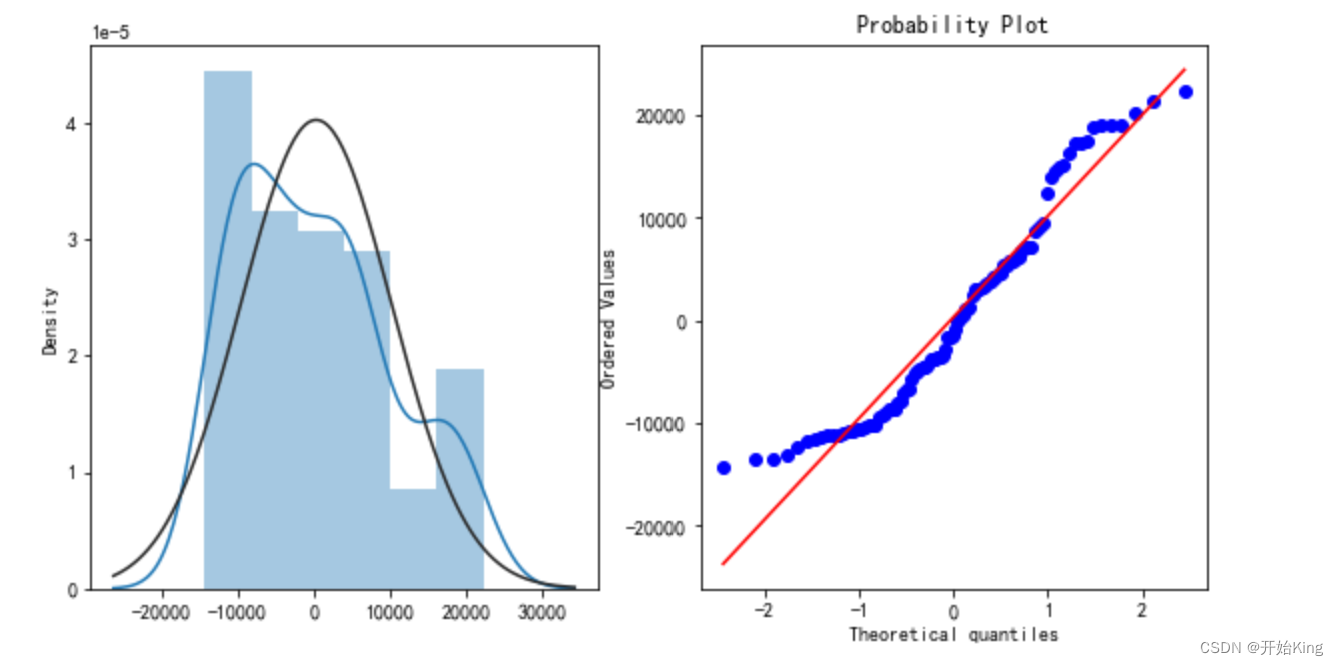
残差正态性检验

import seaborn as sns
from scipy import stats
plt.figure(figsize=(10,5))
ax=plt.subplot(1,2,1)
sns.distplot(residual,fit=stats.norm)
ax=plt.subplot(1,2,2)
res=stats.probplot(residual,plot=plt)
plt.show()

在开头说过，ARIMA不适用长期预测，下面把预测范围调大，看看是否和文章开头所说的一致

predict=arima_res.predict("2018/1/14 0:00:00","2018/1/18 23:45:00")

plt.plot(range(len(predict)),predict)
plt.legend(['y_true','y_pred'])
plt.show()
print(len(predict))