---

这次我们尝试用支持向量机（SVM）来完成对鸢尾花的分类任务。
对于啥时SVM，我们可以看看一个短视频大概有个了解：【五分钟机器学习】向量支持机SVM: 学霸中的战斗机

一、数据准备

本文所用数据集：《鸢尾花数据集 iris.data》
我们可以先看一下这个数据集里面是啥样子：

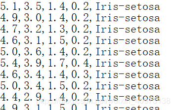
可以看到数据集里面每行有5种数据，分别是萼片长度、萼片宽度、花瓣长度、花瓣宽度和所属类别，其用逗号隔开。

import numpy as np
from sklearn import svm
from sklearn import model_selection
import matplotlib.pyplot as plt
import matplotlib as mpl

file_path = "C:/Users/Noah/Desktop/iris.data"

# 该方法可将输入的字符串作为字典it 的键进行查询，输出对应的值
def iris_type(s):
    it = {b'Iris-setosa':0, b'Iris-versicolor':1, b'Iris-virginica':2}
    return it[s]

# 加载data文件，类型为浮点，分隔符为逗号，对第四列也就是data 中的鸢尾花类别这一列的字符串转换为0-2 的浮点数
data = np.loadtxt(file_path, dtype=float, delimiter=',', converters={4:iris_type})

# 对data 矩阵进行分割，从第四列包括第四列开始后续所有列进行拆分
x, y = np.split(data, (4,), axis=1)
# 对x 矩阵进行切片，所有行都取，但只取前两列
x = x[:, 0:2]
print(x)

# 随机分配训练数据和测试数据，随机数种子为1，测试数据占比为0.3
data_train, data_test, tag_train, tag_test = model_selection.train_test_split(x, y, random_state=1, test_size=0.3)

上文中的iris_type 方法相当于一个转换器，将数据中非浮点类型的字符串转化为浮点。实际上就是把数据集中鸢尾花类型的英文名用0-2 的数字进行代替，方便后续模型的训练。

numpy.loadtxt 方法的作用是将文本格式的数据集转化为一个可以进行分割计算等操作的矩阵。
其参数详解：https://numpy.org/doc/stable/reference/generated/numpy.loadtxt.html

np.split 方法的作用是将一个包含四种特征和一种标签的数据集矩阵分割成两个矩阵，其分别是包含四种特征的特征矩阵和包含一种标签的标签矩阵。
其参数详解：https://numpy.org/doc/stable/reference/generated/numpy.split.html

在x = x[:, 0:2] 这行代码中，我们对特征矩阵进行再一次分割，并只取其前两种特征（萼片长度和萼片宽度），在后续的模型训练过程中，我们都将只使用这两种特征进行训练。
若将此处x = x[:, 0:2] 改为x = x[:, 2:4] 则代表取后两种特征（花瓣长度和花瓣宽度）进行训练。

最后，我们利用model_selection.train_test_split 方法对前面处理好的数据集进行划分，分为训练集和测试集。
其参数详解：https://scikit-learn.org/0.18/modules/generated/sklearn.model_selection.train_test_split.html

二、模型搭建

def classifier():
    clf = svm.SVC(C=0.5,                            # 误差惩罚系数，默认1
                  kernel='linear',                  # 线性核
                  decision_function_shape='ovr')    # 决策函数
    return clf

# 定义SVM（支持向量机）模型
clf = classifier()

svm.SVC 方法其参数详解：
https://scikit-learn.org/stable/modules/generated/sklearn.svm.SVC.html

其中惩罚系数C 越大，对误分类的惩罚增大，趋向于对训练集全分对的情况，这样对训练集测试时准确率很高，但泛化能力弱，也就是容易过拟合。

C值小，对误分类的惩罚减小，允许容错，将他们当成噪声点，泛化能力较强。

kernel 参数表示核函数，其可以简化SVM 中的运算。常用的有三种：线性核linear、高斯核函数rbf、多项式核函数poly。

decision_function_shape 表示决策函数（样本到分离超平面的距离）的类型。

三、模型训练

def train(clf, x_train, y_train):
    clf.fit(x_train,            # 训练集特征向量
            y_train.ravel())    # 训练集目标值

# 训练SVM 模型
train(clf, data_train, tag_train)

四、模型评估

def show_accuracy(a, b, tip):
    acc = a.ravel() == b.ravel()
    print('%s Accuracy:%.3f' % (tip, np.mean(acc)))

在acc = a.ravel() == b.ravel() 中会生成一个矩阵acc，其中每个元素都是True 或False，而np.mean(acc) 则会计算出这个矩阵的均值，也就是正确率。

def print_accuracy(clf, x_train, y_train, x_test, y_test):
    # 分别打印训练集和测试集的准确率
    print('training prediction:%.3f' % (clf.score(x_train, y_train)))
    print('test data prediction:%.3f' % (clf.score(x_test, y_test)))
    # 原始结果与预测结果进行对比
    show_accuracy(clf.predict(x_train), y_train, 'training data')
    show_accuracy(clf.predict(x_test), y_test, 'testing data')
    # 计算决策函数的值，表示x到各分割平面的距离
    print('decision_function:\n', clf.decision_function(x_train))

其中score(x_train, y_train) 表示输出x_train, y_train 在模型上的准确率，predict(x_train) 表示对x_train 样本进行预测，返回样本类别。

print_accuracy(clf, data_train, tag_train, data_test, tag_test)

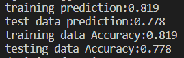
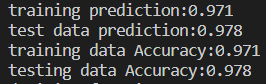
执行该方法后，可见两个show_accuracy() 方法计算出来的结果与两个clf.score() 所得结果相同：

五、数据可视化

def draw(clf, x):
    iris_feature = 'sepal length', 'sepal width', 'petal length', 'petal width'
    # 开始画图
    # 第0 列的范围
    x1_min, x1_max = x[:, 0].min(), x[:, 0].max()
    # 第1 列的范围
    x2_min, x2_max = x[:, 1].min(), x[:, 1].max()
    x1, x2 = np.mgrid[x1_min:x1_max:200j, x2_min:x2_max:200j]
    grid_test = np.stack((x1.flat, x2.flat), axis=1)
    print('grid_test:\n', grid_test)
    # 输出样本到决策面的距离
    z = clf.decision_function(grid_test)
    print('the distance to decision plane:\n', z)
    # 预测分类值
    grid_hat = clf.predict(grid_test)
    print('grid_hat:\n', grid_hat)
    grid_hat = grid_hat.reshape(x1.shape)

    cm_light = mpl.colors.ListedColormap(['#A0FFA0', '#FFA0A0', '#A0A0FF'])
    cm_dark = mpl.colors.ListedColormap(['g', 'r', 'b'])

    plt.pcolormesh(x1, x2, grid_hat, cmap=cm_light)
    # 样本点
    plt.scatter(x[:, 0], x[:, 1], c=np.squeeze(y), edgecolor='k', s=50, cmap=cm_dark)
    # 测试点
    plt.scatter(data_test[:, 0], data_test[:, 1], s=120, facecolor='none', zorder=10)
    plt.xlabel(iris_feature[0], fontsize=20)
    plt.ylabel(iris_feature[1], fontsize=20)
    plt.xlim(x1_min, x1_max)
    plt.ylim(x2_min, x2_max)
    plt.title('svm in iris data classification', fontsize=30)
    plt.grid()
    plt.show()

draw(clf, x)

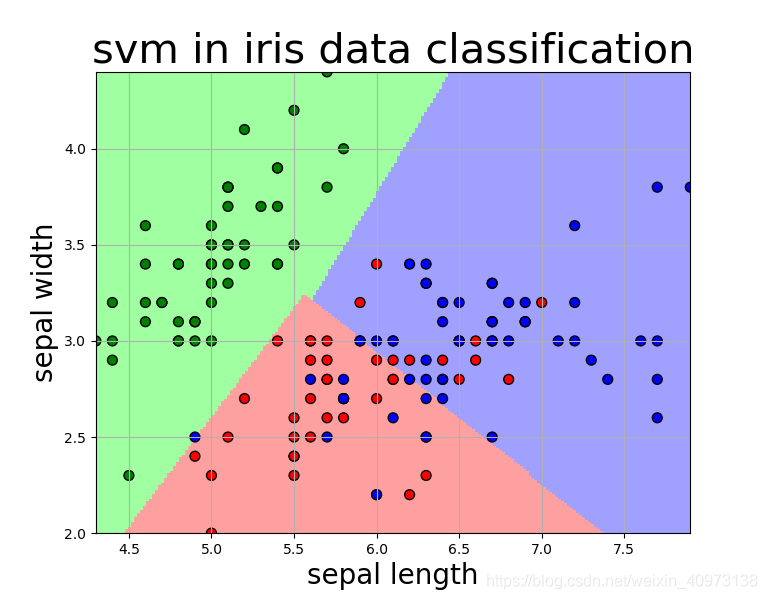
我们可以看到，仅依靠萼片长度和萼片宽度作为两种特征进行模型训练，在Iris-versicolor（红点所示） 与Iris-virginica（蓝点所示） 之间并不能达到很好的分类效果。

但是如果我们选取的是花瓣长度和花瓣宽度作为特征进行训练，则情况就完全不一样了：

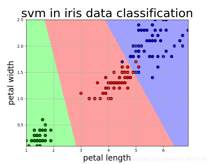
我们可以看到，三种鸢尾花在花瓣长度和花瓣宽度上具有很好的分辨度，该模型基本可以实现很好的分类效果，除了有两个红点分布在了蓝色区域，我们可以认为其是离群点。

这是该模型的准确度：

六、完整代码

import numpy as np
from sklearn import svm
from sklearn import model_selection
import matplotlib.pyplot as plt
import matplotlib as mpl

#=============== 数据准备 ===============
file_path = "C:/Users/waao_wuyou/Desktop/iris.data"

# 该方法可将输入的字符串作为字典it 的键进行查询，输出对应的值
# 该方法就是相当于一个转换器，将数据中非浮点类型的字符串转化为浮点
def iris_type(s):
    it = {b'Iris-setosa':0, b'Iris-versicolor':1, b'Iris-virginica':2}
    return it[s]

# 加载data文件，类型为浮点，分隔符为逗号，对第四列也就是data 中的鸢尾花类别这一列的字符串转换为0-2 的浮点数
data = np.loadtxt(file_path, dtype=float, delimiter=',', converters={4:iris_type})
# print(data)

# 对data 矩阵进行分割，从第四列包括第四列开始后续所有列进行拆分
x, y = np.split(data, (4,), axis=1)
# 对x 矩阵进行切片，所有行都取，但只取前两列
x = x[:, 0:2]
print(x)

# 随机分配训练数据和测试数据，随机数种子为1，测试数据占比为0.3
data_train, data_test, tag_train, tag_test = model_selection.train_test_split(x, y, random_state=1, test_size=0.3)

#=============== 模型搭建 ===============
def classifier():
    clf = svm.SVC(C=0.5,                            # 误差惩罚系数，默认1
                  kernel='linear',                  # 线性核 kenrel='rbf':高斯核
                  decision_function_shape='ovr')    # 决策函数
    return clf

# 定义SVM（支持向量机）模型
clf = classifier()

#=============== 模型训练 ===============
def train(clf, x_train, y_train):
    clf.fit(x_train,            # 训练集特征向量
            y_train.ravel())    # 训练集目标值

# 训练SVM 模型
train(clf, data_train, tag_train)

#=============== 模型评估 ===============
def show_accuracy(a, b, tip):
    acc = a.ravel() == b.ravel()
    print('%s Accuracy:%.3f' % (tip, np.mean(acc)))

def print_accuracy(clf, x_train, y_train, x_test, y_test):
    # 分别打印训练集和测试集的准确率
    # score(x_train, y_train):表示输出x_train, y_train 在模型上的准确率
    print('training prediction:%.3f' % (clf.score(x_train, y_train)))
    print('test data prediction:%.3f' % (clf.score(x_test, y_test)))
    # 原始结果与预测结果进行对比
    # predict() 表示对x_train 样本进行预测，返回样本类别
    show_accuracy(clf.predict(x_train), y_train, 'training data')
    show_accuracy(clf.predict(x_test), y_test, 'testing data')
    # 计算决策函数的值，表示x到各分割平面的距离
    print('decision_function:\n', clf.decision_function(x_train))

print_accuracy(clf, data_train, tag_train, data_test, tag_test)

#=============== 模型可视化 ===============
def draw(clf, x):
    iris_feature = 'sepal length', 'sepal width', 'petal length', 'petal width'
    # 开始画图
    # 第0 列的范围
    x1_min, x1_max = x[:, 0].min(), x[:, 0].max()
    # 第1 列的范围
    x2_min, x2_max = x[:, 1].min(), x[:, 1].max()
    x1, x2 = np.mgrid[x1_min:x1_max:200j, x2_min:x2_max:200j]
    grid_test = np.stack((x1.flat, x2.flat), axis=1)
    print('grid_test:\n', grid_test)
    # 输出样本到决策面的距离
    z = clf.decision_function(grid_test)
    print('the distance to decision plane:\n', z)
    # 预测分类值
    grid_hat = clf.predict(grid_test)
    print('grid_hat:\n', grid_hat)
    grid_hat = grid_hat.reshape(x1.shape)

    cm_light = mpl.colors.ListedColormap(['#A0FFA0', '#FFA0A0', '#A0A0FF'])
    cm_dark = mpl.colors.ListedColormap(['g', 'r', 'b'])

    plt.pcolormesh(x1, x2, grid_hat, cmap=cm_light)
    # 样本点
    plt.scatter(x[:, 0], x[:, 1], c=np.squeeze(y), edgecolor='k', s=50, cmap=cm_dark)
    # 测试点
    plt.scatter(data_test[:, 0], data_test[:, 1], s=120, facecolor='none', zorder=10)
    plt.xlabel(iris_feature[0], fontsize=20)
    plt.ylabel(iris_feature[1], fontsize=20)
    plt.xlim(x1_min, x1_max)
    plt.ylim(x2_min, x2_max)
    plt.title('svm in iris data classification', fontsize=30)
    plt.grid()
    plt.show()

draw(clf, x)