如何将数据指标异常监控和归因分析自动化
数据指标异常波动是产品运营以及数据分析相关岗位日常工作中较为常见的问题之一,及时监控核心指标异常波动并预警,有助于业务快速定位和发现问题(归因分析),或者捕捉业务异动信息,把握市场机会。建立完善的指标异常监控与归因方案,能够提高监控和归因的效率和准确性。本篇文章主要介绍指标异常监控和归因方案。...
目录
一、数据指标监控与归因目的
数据指标异常波动是产品运营以及数据分析相关岗位日常工作中较为常见的问题之一,及时监控核心指标异常波动并预警,有助于业务快速定位和发现问题(归因分析),或者捕捉业务异动信息,把握市场机会。建立完善的指标异常监控与归因方案,能够提高监控和归因的效率和准确性。本篇文章主要介绍指标异常监控和归因方案。
二、监控与归因框架
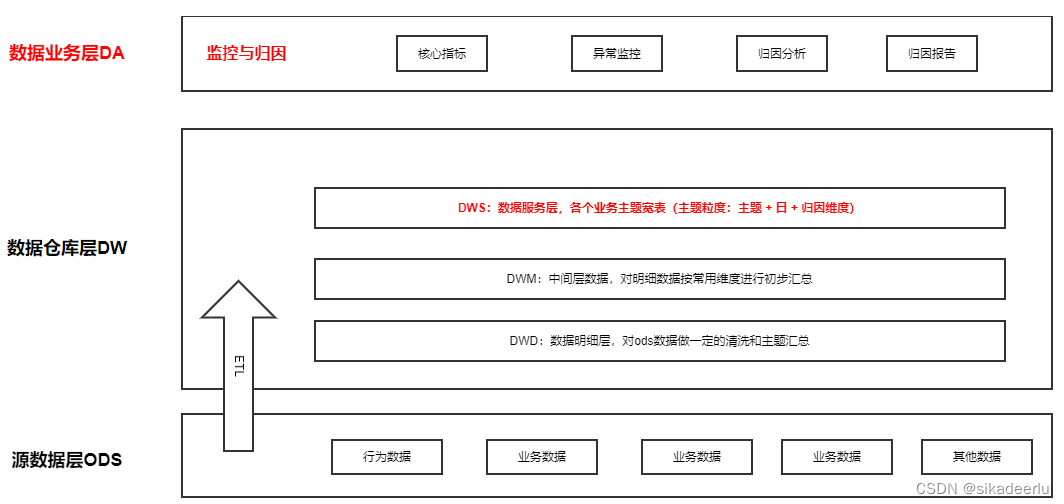
监控与归因是基于数仓建设的上层具体应用,进行指标监控需要有每日核心指标维度的数据,进行归因需要底层有待归因维度的数据建设,对底层数据进行适当的建模是监控分析的第一步。
下图是基于数仓建设的监控与归因方案框架,
三、指标监控方法与实施
3.1 指标异常监控方法
这里以APP日活指标为例,对异常归因方法进行说明
1、阈值方法
a.固定阈值法:如日活大于或者小于固定值时进行异常预警;
b.同环比阈值法:如日活环比上周同期波动大于或者小于固定百分比时进行异常预警;
2、统计方法
a.2/3倍标准差法:我们知道正态分布中,数据分布在2倍标准差内的概率是95.5%,在3倍标准差的概率内是99.7%,因此如果日活大于或小于过1个月日活均值的2倍标准差(如果数据有明显的按周波动,可按星期往前推,如目前是周五,考察前5个周五的均值和标准差,并进行对比),则可认为数据异常波动。
b.1.5倍IQR:和标准差类似,该方法是基于箱线图进行异常判断。
3、建模方法
首先对指标进行建模进行预测,基于实际值和预测值的偏离来进行异常监控,该方法会更灵活,当然所需要的时间也更多。
a.时间序列法:时间序列主要有两种方法,一种效应分解法,主要参考facebook的prophet方法进行建模;另外一种是基于宽平稳时间序列统计方法预测方法ARIMA,AR代表自回归模型、I代表差分、MA代表移动平均模型,python中的statsmodel中tsa.arima_model可进行预测。
b.长短时记忆网络LSTM
3.2 梳理核心监控指标并进行异常监控
1、梳理业务核心KPI,如日活、交易量公司级别重点关注的指标
2、对核心指标进行底层数据建模(日维度汇总、日+归因维度汇总)
3、以2倍标准差为例判断是否异常:计算当前日期前N天(也可以更细的粒度当前日期如果是周三,计算前N个周三)的均值、标准差、2倍标准差的上线限分别是多少,如果当日指标在2倍标准差范围之外,则判断为异常波动,并检验监测结果是否真正异常,从而不断优化异常监控方案。
四、异常归因方法与实施
4.1 Adtributor根因分析原理介绍
a.首先计算各个维度下,各个值的 预测值占整体预测值的比例 , 各个值的 实际值占整体预测值的比例, 利用js散度计算预测分布和实际分布的差异,js值越大,差异程度越大,js散度的计算公式如下:


b.计算某维度下某因素波动占总体波动的比例,并按降序排列
c.对差异程度进行排序,确定根因所在的维度,并给出维度内部每个元素的解释力
4.2 Adtributor根因分析python代码示例
以日活的异常波动为例进行根因分析,现有3月-5月的日活整体数据、日活按城市、机型两个维度拆解的共三份数据集,下边代码是异常监控及根因分析代码。所用数据部分链接如下(数据可能和下文有差异,不影响用来练习测试):https://download.csdn.net/download/baidu_26137595/87177452
############ 1、数据读取 ############
# 整体日活
data = pd.read_excel('./dau.xlsx', sheet_name = '日活')
dau_app = data[data['渠道'] == 'App']

# 按城市日活
data_city = pd.read_excel('./dau.xlsx', sheet_name = '日活按城市拆分')
dau_city_app = data_city[data_city['渠道'] == 'App']

# 按机型日活
data_manu = pd.read_excel('./dau.xlsx', sheet_name = '日活按机型拆分')
dau_manu_app = data_manu[data_manu['渠道'] == 'App']


############ 2、数据预处理 ############
# 添加星期
dau_app = dau_app.sort_values(by = ['date'])  # 按照日期进行排序
dau_app['weekday'] = dau_app['date'].apply(lambda x: x.weekday() + 1)  # 添加星期

dau_manu_app = dau_manu_app.sort_values(by = ['date'])  # 按照日期进行排序
dau_manu_app['weekday'] = dau_manu_app['date'].apply(lambda x: x.weekday() + 1)  # 添加星期

dau_city_app = dau_city_app.sort_values(by = ['date'])  # 按照日期进行排序
dau_city_app['weekday'] = dau_city_app['date'].apply(lambda x: x.weekday() + 1)  # 添加星期


############ 3、获取历史数据的均值、标准差信息 ############
# 定义函数:获取整体日活历史5周日活的均值、标准差信息
def get_his_week_dau_ms( currdate, xdaysbefcurr, currweek, dau_app):
    thred = {}  # 这里注意dict的赋值方式

    dau_app_bef_35d = dau_app[(dau_app['date'] >= xdaysbefcurr) & (dau_app['date'] < currdate) & (dau_app['weekday'] == currweek)]

    thred['deta'] = dau_app_bef_35d
    thred['mean'] = dau_app_bef_35d['user_num1'].mean()
    thred['std'] = dau_app_bef_35d['user_num1'].std()
    thred['std_1_lower'] = dau_app_bef_35d['user_num1'].mean() - dau_app_bef_35d['user_num1'].std()
    thred['std_1_upper'] = dau_app_bef_35d['user_num1'].mean() + dau_app_bef_35d['user_num1'].std()
    thred['std_2_lower'] = dau_app_bef_35d['user_num1'].mean() - 2 * dau_app_bef_35d['user_num1'].std()
    thred['std_2_upper'] = dau_app_bef_35d['user_num1'].mean() + 2 * dau_app_bef_35d['user_num1'].std()
    thred['std_3_lower'] = dau_app_bef_35d['user_num1'].mean() - 3 * dau_app_bef_35d['user_num1'].std()
    thred['std_3_upper'] = dau_app_bef_35d['user_num1'].mean() + 3 * dau_app_bef_35d['user_num1'].std()
    return thred


# 定义函数:获取按城市日活历史5周日活的均值、标准差信息
def get_his_week_city_dau_ms( currdate, xdaysbefcurr, currweek, city, dau_app):
    thred = {}  # 这里注意dict的赋值方式

    # 获取当前版本历史周对应的信息
    dau_app_bef_35d = dau_app[(dau_app['date'] >= xdaysbefcurr) & (dau_app['date'] < currdate) & (dau_app['weekday'] == currweek) & (dau_app['$city'] == city)]

    thred['deta'] = dau_app_bef_35d
    thred['mean'] = dau_app_bef_35d['user_num1'].mean()
    thred['std'] = dau_app_bef_35d['user_num1'].std()
    thred['std_1_lower'] = dau_app_bef_35d['user_num1'].mean() - dau_app_bef_35d['user_num1'].std()
    thred['std_1_upper'] = dau_app_bef_35d['user_num1'].mean() + dau_app_bef_35d['user_num1'].std()
    thred['std_2_lower'] = dau_app_bef_35d['user_num1'].mean() - 2 * dau_app_bef_35d['user_num1'].std()
    thred['std_2_upper'] = dau_app_bef_35d['user_num1'].mean() + 2 * dau_app_bef_35d['user_num1'].std()
    thred['std_3_lower'] = dau_app_bef_35d['user_num1'].mean() - 3 * dau_app_bef_35d['user_num1'].std()
    thred['std_3_upper'] = dau_app_bef_35d['user_num1'].mean() + 3 * dau_app_bef_35d['user_num1'].std()
    return thred

# 定义函数:获取按机型日活历史5周日活的均值、标准差信息
def get_his_week_manu_dau_ms( currdate, xdaysbefcurr, currweek, manu, dau_app):
    thred = {}  # 这里注意dict的赋值方式

    # 获取当前版本历史周对应的信息
    dau_app_bef_35d = dau_app[(dau_app['date'] >= xdaysbefcurr) & (dau_app['date'] < currdate) & (dau_app['weekday'] == currweek) & (dau_app['$manufacturer'] == manu)]

    thred['deta'] = dau_app_bef_35d
    thred['mean'] = dau_app_bef_35d['user_num1'].mean()
    thred['std'] = dau_app_bef_35d['user_num1'].std()
    thred['std_1_lower'] = dau_app_bef_35d['user_num1'].mean() - dau_app_bef_35d['user_num1'].std()
    thred['std_1_upper'] = dau_app_bef_35d['user_num1'].mean() + dau_app_bef_35d['user_num1'].std()
    thred['std_2_lower'] = dau_app_bef_35d['user_num1'].mean() - 2 * dau_app_bef_35d['user_num1'].std()
    thred['std_2_upper'] = dau_app_bef_35d['user_num1'].mean() + 2 * dau_app_bef_35d['user_num1'].std()
    thred['std_3_lower'] = dau_app_bef_35d['user_num1'].mean() - 3 * dau_app_bef_35d['user_num1'].std()
    thred['std_3_upper'] = dau_app_bef_35d['user_num1'].mean() + 3 * dau_app_bef_35d['user_num1'].std()
    return thred

# 添加整体日活的波动信息
for index, row in dau_app.iterrows():
#     print(row)
    currdate = row['date']
    xdaysbefcurr = row['date'] - datetime.timedelta(days = 35)
    currweek = row['weekday']

#     print('--', currdate, xdaysbefcurr, currweek)
    tmp = get_his_week_dau_ms(currdate, xdaysbefcurr, currweek,  dau_app)
    dau_app.at[index, 'his_mean'] = tmp['mean']
    dau_app.at[index, 'his_std'] = tmp['std']
    dau_app.at[index, 'std_1_lower'] = tmp['std_1_lower']
    dau_app.at[index, 'std_1_upper'] = tmp['std_1_upper']
    dau_app.at[index, 'std_2_lower'] = tmp['std_2_lower']
    dau_app.at[index, 'std_2_upper'] = tmp['std_2_upper']
    dau_app.at[index, 'std_3_lower'] = tmp['std_3_lower']
    dau_app.at[index, 'std_3_upper'] = tmp['std_3_upper']

# 添加按城市日活的历史波动信息
for index, row in dau_city_app.iterrows():
    currdate = row['date']
    xdaysbefcurr = row['date'] - datetime.timedelta(days = 35)
    currweek = row['weekday']
    city = row['$city']
#     print('--', currdate, xdaysbefcurr, currweek)
    tmp = get_his_week_city_dau_ms(currdate, xdaysbefcurr, currweek, city, dau_city_app)


    dau_city_app.at[index, 'his_mean'] = tmp['mean']
    dau_city_app.at[index, 'his_std'] = tmp['std']
    dau_city_app.at[index, 'std_1_lower'] = tmp['std_1_lower']
    dau_city_app.at[index, 'std_1_upper'] = tmp['std_1_upper']
    dau_city_app.at[index, 'std_2_lower'] = tmp['std_2_lower']
    dau_city_app.at[index, 'std_2_upper'] = tmp['std_2_upper']
    dau_city_app.at[index, 'std_3_lower'] = tmp['std_3_lower']
    dau_city_app.at[index, 'std_3_upper'] = tmp['std_3_upper']

# 添加按机型日活的历史波动信息
for index, row in dau_manu_app.iterrows():
    currdate = row['date']
    xdaysbefcurr = row['date'] - datetime.timedelta(days = 35)
    currweek = row['weekday']
    manu = row['$manufacturer']
#     print('--', currdate, xdaysbefcurr, currweek)
    tmp = get_his_week_manu_dau_ms(currdate, xdaysbefcurr, currweek, manu, dau_manu_app)

    dau_manu_app.at[index, 'his_mean'] = tmp['mean']
    dau_manu_app.at[index, 'his_std'] = tmp['std']
    dau_manu_app.at[index, 'std_1_lower'] = tmp['std_1_lower']
    dau_manu_app.at[index, 'std_1_upper'] = tmp['std_1_upper']
    dau_manu_app.at[index, 'std_2_lower'] = tmp['std_2_lower']
    dau_manu_app.at[index, 'std_2_upper'] = tmp['std_2_upper']
    dau_manu_app.at[index, 'std_3_lower'] = tmp['std_3_lower']
    dau_manu_app.at[index, 'std_3_upper'] = tmp['std_3_upper']

############ 4、判断是否异常 ############
def get_if_abnormal(x):
#     print(x)
    flag = 0 # 默认为0,即为正常波动
    # 如果 历史均值 his_mean 不为nan ,且 当前日活在 2倍标准差之外,则为异常波动
    if pd.isna(x['his_mean']):
        return flag
    elif x['user_num1'] > x['std_2_upper'] or  x['user_num1'] < x['std_2_lower']:
        flag = 1
    return flag
dau_app['is_abnormal'] = dau_app.apply(lambda x: get_if_abnormal(x), axis = 1)
dau_app[dau_app['is_abnormal'] == 1] # 查看被标记为异常的数据

############ 5、Adtributor根因分析 ############
##### 5.1 定义函数:首先计算js散度所需要的两个值,预测值占比和实际值占比
def get_js_detail_info(row_dim, row_all):
    js_detail = {}

    # 计算该水平下实际值占整体值的比例
    if pd.isna(row_dim.user_num1) or pd.isna(row_all.user_num1):
        real_pct = None
    else:
        real_pct = row_dim.user_num1/row_all.user_num1

    # 计算该水平下预测值占整体预测值的比例
    if pd.isna(row_dim.his_mean) or pd.isna(row_all.his_mean):
        pred_pct = None
    else:
        pred_pct = row_dim.his_mean/row_all.his_mean

    # 计算该水平实际值-预测值 占 整体实际值-预测值的 比例
    if pd.isna(row_dim.his_mean) or pd.isna(row_all.his_mean) or pd.isna(row_dim.user_num1) or pd.isna(row_all.user_num1):
        diff_pct = None
    else:
        diff_pct = (row_dim.user_num1 - row_dim.his_mean)/(row_all.user_num1 - row_all.his_mean)

    js_detail['real_pct'] = real_pct
    js_detail['pred_pct'] = pred_pct
    js_detail['diff_pct'] = diff_pct
    return js_detail

# 按城市日活添加 实际占比 和 预测占比
for index, row in dau_city_app_copy.iterrows():

    row_all = dau_app[dau_app['date'] == row.date]
    row_all = pd.Series(row_all.values[0], index = row_all.columns)  # dataframe类型转为series类型

    js_detail = get_js_detail_info(row, row_all)

    print('js_detail', js_detail)
    dau_city_app_copy.at[index, 'real_pct'] = js_detail['real_pct']
    dau_city_app_copy.at[index, 'pred_pct'] = js_detail['pred_pct']
    dau_city_app_copy.at[index, 'diff_pct'] = js_detail['diff_pct']

# 按机型日活添加 实际占比和预测占比
for index, row in dau_manu_app_copy.iterrows():
    row_all = dau_app[dau_app['date'] == row.date]
    row_all = pd.Series(row_all.values[0], index = row_all.columns)  # dataframe类型转为series类型

    js_detail = get_js_detail_info(row, row_all)

    print('js_detail', js_detail)
    dau_manu_app_copy.at[index, 'real_pct'] = js_detail['real_pct']
    dau_manu_app_copy.at[index, 'pred_pct'] = js_detail['pred_pct']
    dau_manu_app_copy.at[index, 'diff_pct'] = js_detail['diff_pct']

##### 5.2 定义函数计算js散度
def get_js_divergence(p, q):
    p = np.array(p)
    q = np.array(q)
    M = (p + q)/2

    js1 = 0.5 * np.sum(p * np.log(p/M))+ 0.5 *np.sum(q* np.log(q/M))  # 自己计算
    js2 = 0.5 * stats.entropy(p, M) + 0.5 * stats.entropy(q, M)    # scipy包中方法
    print('js1', js1)
    print('js2', js2)
    return round(float(js2),4)

##### 5.3 以4月24日日活波动异常为例从城市和机型维度进行归因
tmp = dau_city_app_copy[dau_city_app_copy['date'] == '2022-04-24'].dropna()
get_js_divergence(tmp['real_pct'], tmp['pred_pct'])
# js1: 0.014734253529123373  js2:  0.013824971768932472

tmp2 = dau_manu_app_copy[dau_manu_app_copy['date'] == '2022-04-24'].dropna()
get_js_divergence(tmp2['real_pct'], tmp2['pred_pct'])
# js1: 6.915922987763717e-05  js2:  6.9049339769412e-05 (约0.00010)
# 由此得出城市维度是异常波动的原因,查看当天城市维度的明细数据
tmp.sort_values(by = 'diff_pct', ascending = False,)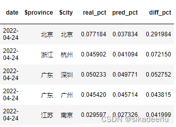
从城市维度的数据可以看到,北京在4月24日当天的日活实际占整体日活比例为0.0772,按照历史数据预测的话占比为0.0378,北京当天的波动占整体日活的波动为29.20%,结合近期疫情情况推测主要由于北京近期疫情反复造成的业务波动。
4.3 Adtributor根因分析hive实现核心代码
这里以地区维度为例看如何在hive中实现。其中j计算s散度用到的预测值以及差异计算相对指标都用上周同期数据即前7天数据,这个基准值可根据需要进行调整。
-- 1.各地区每日指标
drop table db.area_cnt;
create table db.area_cntstored as parquet as
select area_name area_name
, count(1) cnt --单量
, count(distinct user_id) user_num -- 用户数
, inc_day
from db.area_dtl t
where inc_day >= replace(date_sub('${lastday}', 15), '-', '')
and inc_day <= replace('${lastday}', '-', '')
group by area_name
, inc_day;
-- 2.保存按地区汇总数据
insert overwrite table db.area_cnt_di partition(inc_day)
select area_name, cnt, user_num, inc_day
from db.area_cnt
union all
select '整体' area_name, sum(cnt) cnt, sum(user_num ) user_num , inc_day
from db.area_cnt
group by inc_day;
-- 3.计算各地区前7天数据
drop table if exists db.area_cnt_di_01 ;
create table db.area_cnt_di_01 stored as parquet as
select t.inc_day
, t.area_name
, t.cnt
, t1.cnt cnt_b7 -- 前7天
, t.cnt - t1.cnt cnt_b7_diff
from (
select t0.*
, date_sub(inc_day, 7) inc_day_new_b7 -- 上周数据
from db.area_cnt_di t0
where inc_day >= date_sub('${lastday}', 15)
and inc_day <= '${lastday}'
) t
left join db.area_cnt_di t1
on t.inc_day_new_b7 = t1.inc_day and t.area_name = t1.area_name;
-- 4.计算实际占比和波动占比,并计算js散度
drop table if exists db.area_cnt_di_02 ;
create table db.area_cnt_di_02 stored as parquet as
select t.*
, log(2.7182818, 2*cnt_pct/(cnt_pct + cnt_b7_pct)) px_f1 -- px log部分计算结果
, log(2.7182818, 2*cnt_b7_pct/(cnt_pct + cnt_b7_pct)) qx_f1 -- qx log部分计算结果
, 0.5*cnt_pct*log(2.7182818, 2*cnt_pct/(cnt_pct + cnt_b7_pct)) + 0.5*cnt_b7_pct*log(2.7182818, 2*cnt_b7_pct/(cnt_pct + cnt_b7_pct)) js_value
from (
select
t.inc_day
, t.area_name
-- 该地区数据
, t.cnt
, t.cnt_b7
, t.cnt_b7_diff
-- 整体数据
, t1.cnt all_cnt
, t1.cnt_b7 all_cnt_b7
, t1.cnt_b7_diff all_cnt_b7_diff
-- 各地区与整体数据
, t.cnt/t1.cnt cnt_pct -- 当日各地区占比
, t.cnt_b7/t1.cnt_b7 cnt_b7_pct -- 上周各地区占比
, t.cnt_b7_diff/t1.cnt_b7_diff diff_pct -- 差异占整体比例是多少
from db.area_cnt_di_01 t -- 各地区数据
left join (
select area_name, inc_day, cnt, cnt_b7, cnt_b7_diff
from db.area_cnt_di_01
where area_name = '整体'
) t1 -- 整体数据
on t.inc_day = t1.inc_day
) t
;
-- 5. 并计算每一天的js散度
drop table if exists db.area_cnt_di_03 ;
create table db.area_cnt_di_03 stored as parquet as
select t.inc_day
, sum(js_value) js_value
from db.area_cnt_di_02 t
where area_name <> '整体'
group by inc_day;
-- 6. 合并数据,并计算各地区贡献度排名
drop table if exists db.area_cnt_di_04 ;
create table db.area_cnt_di_04 stored as parquet as
select inc_day
, area_name
, cnt
, cnt_b7
, cnt_b7_diff
, all_cnt
, all_cnt_b7
, all_cnt_b7_diff
, cnt_pct
, cnt_b7_pct
, diff_pct
, row_number() over(partition by inc_day order by diff_pct desc) diff_pct_rn
, px_f1
, qx_f1
, js_value
from db.area_cnt_di_03
where area_name <> '整体'
union all
select t.inc_day
, t.area_name
, t.cnt
, t.cnt_b7
, t.cnt_b7_diff
, t.all_cnt
, t.all_cnt_b7
, t.all_cnt_b7_diff
, t.cnt_pct
, t.cnt_b7_pct
, t.diff_pct
, 1 diff_pct_rn
, t.px_f1
, t.qx_f1
, t1.js_value
from db.area_cnt_di_03 t
left join db.area_cnt_di_03 t1
on t.inc_day = t1.inc_day
where area_name = '整体'
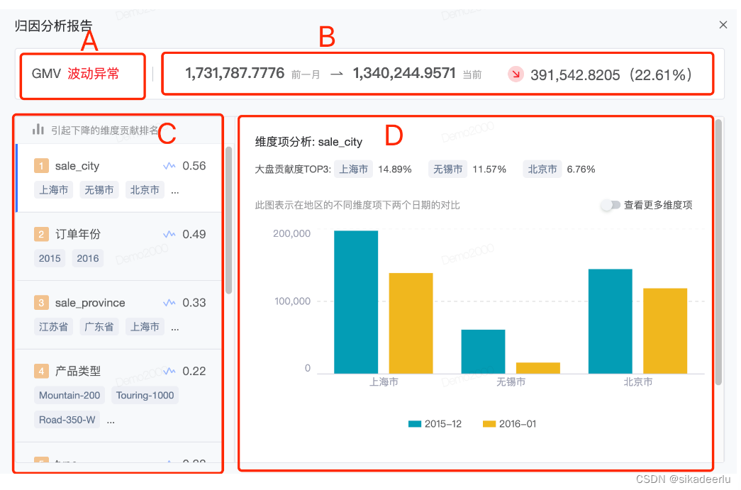
;五、智能归因可视化
有了以上整体指标波动数据、各维度js散度、各维度下各因素(维度项)的实际达成、预期达成、差异贡献度等各项数据,就可以根据这些数据搭建智能归因看板。这里可参考火山引擎的智能归因模块,进行整体可视化效果展示。
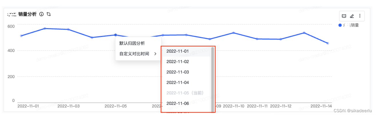
5.1 整体指标波动情况
首先是整体指标达成情况,可单独展示波动情况,也可根据需要展示相关核心指标。点击某天,可展示当天的归因结论。
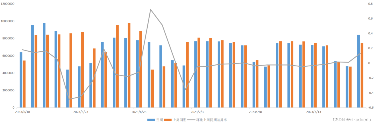
也可将当期(实际值)、上周同期(预期值)、差异率这几个指标根据需要进行如下可视化展示,能在一张图中看到更多信息:
5.2 归因分析结论
如下A、B部分主要展示指标是否异常波动,以及判断依据。C部分为异常维度定位,可用js散度值进行降序排序,D部分为Top N因素贡献情况,C和D实现点击联动,可查看对应维度的Top N因素。

为开发者提供学习成长、分享交流、生态实践、资源工具等服务,帮助开发者快速成长。
更多推荐


 9
9 0
0- 0


 已为社区贡献1条内容

所有评论(0)